CF5

1. Corporate Finance

CORPORATE FINANCE
Elena Rogova, professor, e.rogova@gsom.spbu.ru
Fall semester, 2025-2026

2. Capital Structure - Definition

• Capital Structure refers to the mix of long-term sources of funds used
by the firm.
• Capital structure should be well planned generally keeping in view the
interest of the equity shareholders and the financial requirements of a
company.
Value of the Firm:
V=D+E
Debt
Equity
01.12.2025
2

3. The Choices in Financing

There are only two ways in which a business can make money
Debt:
The essence of debt is that you
promise to make fixed payments in
the future (interest payments and
repaying principal). If you
fail to make those payments, you lose
control of your business.
01.12.2025
OR
Equity:
With equity, you do get
whatever cash flows are
left over after you have
made debt payments
3

4. Debt: Summarizing the Trade Off

Advantages of Borrowing
Tax Shield
Added Discipline
Disadvantages of Borrowing
Bankruptcy costs
Agency costs
Loss of Future Flexibility
01.12.2025
4

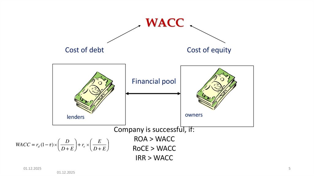
5.

WACC
Cost of debt
Cost of equity
Financial pool
lenders
owners
Company is successful, if:
ROA > WACC
D
E
WACC r (1 )
r
RoCE > WACC
D E
D E
IRR > WACC
d
01.12.2025
e
01.12.2025
5

6. Capital Structure Theories

• The total capital structure theories can be categorised into two relevant
and irrelevant theories.
The following are the main theories/Approaches of capital structure:
1. Net Income Approach
2. Modigliani and Miller Approach
3. Traditional Approach
4. Comparables Approach
01.12.2025
6

7.

Topic 5. Capital
Structure
Optimisation
01.12.2025
Topic 4. Capital
Structure
Theories
7

8. A Framework for Getting to the Optimal

01.12.2025
8

9. Approaches to the Optimal Capital Structure

1. The Cost of Capital Approach: The optimal debt ratio is the one that
minimizes the cost of capital for a firm.
2. The Adjusted Present Value Approach: The optimal debt ratio is the
one that maximizes the overall value of the firm.
3. The Sector Approach: The optimal debt ratio is the one that brings
the firm closes to its peer group in terms of financing mix.
4. The Life Cycle Approach: The optimal debt ratio is the one that best
suits where the firm is in its life cycle.
01.12.2025
9

10. The Cost of Capital Approach

• Value of a Firm = Present Value of Cash Flows to the Firm, discounted
back at the cost of capital.
• If the cash flows to the firm are held constant, and the cost of capital
is minimized, the value of the firm will be maximized.
01.12.2025
10

11. Measuring Cost of Capital

• The cost of debt is the market interest rate that the firm has to pay on its longterm borrowing today, net of tax benefits. It will be a function of:
The long-term risk-free rate
The default spread for the company, reflecting its credit risk
The firm’s marginal tax rate
• The cost of equity reflects the expected return demanded by marginal equity
investors. If they are diversified, only the portion of the equity risk that cannot be
diversified away (beta or betas) will be priced into the cost of equity.
• The cost of capital is the cost of each component weighted by its relative market
value.
Cost of capital (WACC) = Cost of equity (E/(D+E)) + After-tax cost of debt (D/(D+E))
01.12.2025
11

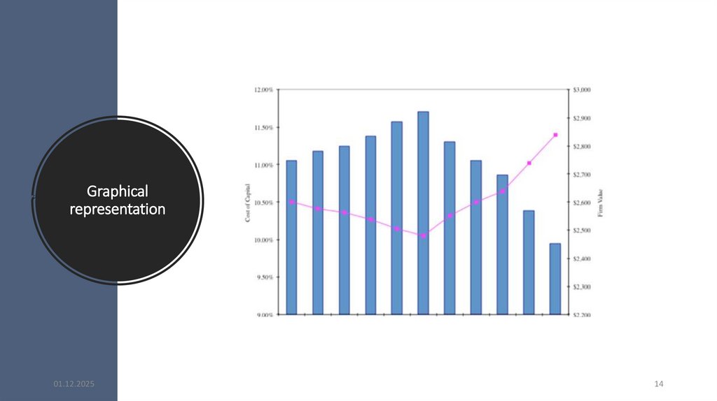
12. Applying Cost of Capital Approach: The Example

Assume the firm has $200 million in cash flows, expected to grow 3% a year forever.
01.12.2025
12

13. Applying Cost of Capital Approach: The Example

Assume the firm has $200 million in cash flows, expected to grow 3% a year forever.
01.12.2025
13

14.

Graphical
representation
01.12.2025
14

15. Current Cost of Capital: Norilsk Nickel

• The beta for NN’s stock in December 2021 was 0.99. The T. bond rate at that time was
2.80%. Using an estimated equity risk premium for Russia of 8.60%, we estimated the
cost of equity for NN:
Cost of Equity = 2.80% + 0.99(8.60%) = 11.31%
• NN’s bond rating in December 2021 was BBB, and based on this rating, the spread is
1.99% and estimated pretax cost of debt for NN is 2.80+1.99 = 4.79%. Using a tax rate of
20%, the after-tax cost of debt for NN:
After-Tax Cost of Debt =4.79% (1 – 0.20) =3.832%
• The cost of capital was calculated using these costs and the weights based on market
values of equity (3,505) and debt (759.7):
Cost of capital = 3.832%*(759.7/(3,505+759.7))+11.31%*(3,505/(3,505+759.7))=9.98%
• Average D/E for 5 years = 0.2329
01.12.2025
15

16. Mechanics of Cost of Capital Estimation

1. Estimate the Cost of Equity at different levels of debt:
Equity will become riskier -> Beta will increase -> Cost of Equity will increase.
Estimation will use levered beta calculation
2. Estimate the Cost of Debt at different levels of debt:
Default risk will go up, and bond ratings will go down as debt goes up -> Cost
of Debt will increase.
To estimating bond ratings, we may use the TIE ratio (EBIT/Interest expense)
3. Estimate the Cost of Capital at different levels of debt
4. Calculate the effect on Firm Value and Stock Price.
01.12.2025
16

17. Cost of equity: estimate the unlevered beta for the firm

• The Regression Beta: One approach is to use the regression beta (0.99) and then
unlever, using the average debt to equity ratio (23.29%) during the period of the
regression.
Unlevered beta = 0.99 / (1 + 0.2329(1 - 0.20))= 0.8345
• The Bottom-up Beta: Alternatively, we can back to the source and estimate it from
the betas of the businesses.
• If the company has several businesses, we calculate the proportion of each business
in the value of the company (using EV/Sales ratio), find unlevered betas for each
business and then weight them
• Simplified approach for NN: use only mining and metals: unlevered beta is 1.19
• 2/3 of the final estimate comes from the regression beta and 1/3 from the bottomup beta
• The final estimate: beta = 0.8325*2/3+1.19*1/3 = 0.952
01.12.2025
17

18. NN’s financials

2021
2020
Revenues, bn rub
EBITDA, bn
Depreciation and amortization
1117
751
290
878
543
87
EBIT
Interest expenses
TIE (Interest Coverage Ratio)
461
63.1
7.31
456
19.7
23.1
CAPEX
FCF
242.9
415.9
103.7
348.1
01.12.2025
18

19. Cost of Equity

Debt ratio D/E
Levered ß
Risk-free
rate
MRP
Cost pf
equity
0%
0%
0.952
2.80%
8.60%
10.99%
10%
11.11%
1.037
2.80%
8.60%
11.72%
20%
25%
1.143
2.80%
8.60%
12.63%
30%
42.86%
1.279
2.80%
8.60%
13.80%
40%
66.67%
1.461
2.80%
8.60%
15.36%
50%
100%
1.715
2.80%
8.60%
17.55%
60%
150%
2.096
2.80%
8.60%
20.83%
70%
233.33%
2.731
2.80%
8.60%
26.29%
80%
400%
4.002
2.80%
8.60%
37.21%
90%
900%
7.813
2.80%
8.60%
69.99%
D
(1 tax rate))
E
CoE rf L MRP
L U (1
01.12.2025
19

20. Assumptions

• In calculating the levered beta in this table, we assumed that all market risk is
borne by the equity investors; this may be unrealistic especially at higher levels of
debt.
• We can also consider an alternative estimate of levered betas that apportions
some of the market risk to the debt:
• levered = u [1+(1-t)D/E] - debt (1-t) D/E
• The beta of debt is based upon the rating of the bond and is estimated by
regressing past returns on bonds in each rating class against returns on a market
index. The levered betas estimated using this approach will generally be lower
than those estimated with the conventional model
01.12.2025
20

21. The Ratings Table

Interest coverage ratio is
> 8.50
6.5 – 8.5
5.5 – 6.5
4.25 – 5.5
3 – 4.25
2.5 -3
2.25 –2.5
2 – 2.25
1.75 -2
1.5 – 1.75
1.25 -1.5
0.8 -1.25
0.65 – 0.8
0.2 – 0.65
<0.2
01.12.2025
Rating is
Aaa/AAA
Aa2/AA
A1/A+
A2/A
A3/ABaa2/BBB
Ba1/BB+
Ba2/BB
B1/B+
B2/B
B3/BCaa/CCC
Ca2/CC
C2/C
D2/D
Spread is
0.40%
0.70%
0.85%
1.00%
1.30%
2.00%
3.00%
4.00%
5.50%
6.50%
7.25%
8.75%
9.50%
10.50%
12.00%
Interest rate
3.20%
3.50%
3.65%
3.80%
4.10%
4.80%
5.80%
6.80%
8.30%
9.30%
10.05%
11.55%
12.30%
13.30%
14.80%
T.Bond rate =2.80%
21

22. Estimating Cost of Debt

Start with the market value of the firm = 3,505.0+759.7 = 4,264.7 bn rubles
D/(D+E)
0.00% 10.00% (Debt to capital)
D/E
0.00% 11.11% (D/E = 10/90 = 0.1111)
Debt
0
426.5 (10% of 4,264.7)
EBITDA
EBIT
Interest
751
461
$0
751
461
14
(Same as 0% debt)
(Same as 0% debt)
(Pre-tax cost of debt * Debt)
Pre-tax TIE
∞
31.3
(EBIT/ Interest Expenses)
Likely Rating
AAA
AA
(From Ratings table)
Pre-tax cost of debt 3.20% 3.50% (Riskless Rate + Spread)
01.12.2025
22

23. Test: Can you do the 30% level?

D/(D + E)
20.00%
D/E
25.00%
Debt
852,9
EBIT
461
Interest expense
41
Interest coverage ratio
11.4
Likely rating
BBB
Pretax cost of debt
4.80%
01.12.2025
Iteration 1
(Debt @BBB rate)
30.00%
Iteration 2
(Debt @BB rate)
30.00%
23

24. Bond Ratings, Cost of Debt and Debt Ratios

Debt
Ratio
0%
10%
20%
30%
40%
50%
60%
70%
80%
90%
$ Debt
0
426.5
852,9
1279.4
1705.9
2132.35
2558.9
2985.3
3411.8
3838.2
01.12.2025
Interest
Expense
0
14.71
40.51
60.77
115.15
143.93
255.9
298.5
417.95
508.56
Interest
Coverage
Ratio
∞
31.3
11.4
7.58
4.00
3.2
1.80
1.54
1.1
0.90
Bond Rating
AAA
AA
A
BBB
BB
BB
BBCC
C
Pre-tax
cost of
debt
3.20%
3.50%
3.80%
4.80%
6.80%
6.80%
10.05%
10.05%
12.30%
13.30%
Tax rate
20%
20%
20%
20%
20%
20%
20%
20%
20%
20%
After-tax
cost of debt
2.56%
2.80%
3.04%
3.84%
5.44%
5.44%
8.04%
8.04%
9.84%
10.64%
24

25. NN’s cost of capital schedule…

…
NN’s cost of capital schedule
Debt ratio
0%
10%
20%
30%
40%
50%
60%
70%
80%
90%
Beta
0,952
1,037
1,143
1,279
1,461
1,715
2,096
2,731
4,002
7,813
Cost of Equity
0,1099
0,1172
0,1263
0,138
0,1536
0,1755
0,2083
0,2629
0,3721
0,6999
Cost of Debt (after tax)
0,0256
0,0280
0,0304
0,0384
0,0544
0,0544
0,0804
0,0804
0,0984
0,1064
WACC
0,1099
0,10828
0,10712
0,10812
0,11392
0,11495
0,13156
0,13515
0,15434
0,16575
Nornikel has capital structure close to optimal
01.12.2025
25

26. Effect on Firm Value – Full Valuation

Step 1: Estimate the cash flows to firm
Step 2: Back out the implied growth rate in the current market value
Growth rate = (Firm Value * Cost of Capital – CF to Firm)/(Firm Value + CF to Firm)
Step 3: Revalue the firm with the new cost of capital
FCFF0 (1 g)
Firm Value
(Cost of Capital -g)
01.12.2025
26

27. What if something goes wrong? The Downside Risk

• Sensitivity to Assumptions
A. “What if” analysis
The optimal debt ratio is a function of our inputs on operating income, tax rates and macro
variables. We could focus on one or two key variables – operating income is an obvious choice –
and look at history for guidance on volatility in that number and ask what if questions.
B. “Economic Scenario” Approach
We can develop possible scenarios, based upon macro variables, and examine the optimal
debt ratio under each one. For instance, we could look at the optimal debt ratio for a cyclical firm
under a boom economy, a regular economy and an economy in recession.
• Constraint on Bond Ratings/ Book Debt Ratios
Alternatively, we can put constraints on the optimal debt ratio to reduce exposure to downside
risk. Thus, we could require the firm to have a minimum rating, at the optimal debt ratio or to
have a book debt ratio that is less than a “specified” value.
01.12.2025
27

28. Limitations of the Cost of Capital approach

• It is static: The most critical number in the entire analysis is the
operating income. If that changes, the optimal debt ratio will
change.
• It ignores indirect bankruptcy costs: The operating income is
assumed to stay fixed as the debt ratio and the rating changes.
• Beta and Ratings: It is based upon rigid assumptions of how
market risk and default risk get borne as the firm borrows
more money and the resulting costs.
01.12.2025
28

29. The APV Approach to Optimal Capital Structure

• In the adjusted present value approach, the value of the firm is written as
the sum of the value of the firm without debt (the unlevered firm) and the
effect of debt on firm value
Firm Value = Unlevered Firm Value + (Tax Benefits of Debt - Expected Bankruptcy Cost
from the Debt)
• The optimal debt level is the one that maximizes firm value
01.12.2025
29

30. Implementing the APV Approach

• Step 1: Estimate the unlevered firm value. This can be done in one of two ways:
• Estimating the unlevered beta, a cost of equity based upon the unlevered beta and valuing the
firm using this cost of equity (which will also be the cost of capital, with an unlevered firm)
• Alternatively, Unlevered Firm Value = Current Market Value of Firm - Tax Benefits of Debt
(Current) + Expected Bankruptcy cost from Debt
• Step 2: Estimate the tax benefits at different levels of debt. The simplest assumption
to make is that the savings are perpetual, in which case
• Tax benefits = Debt * Tax Rate
• Step 3: Estimate a probability of bankruptcy at each debt level, and multiply by the
cost of bankruptcy (including both direct and indirect costs) to estimate the
expected bankruptcy cost.
01.12.2025
30

31. Estimating Expected Bankruptcy Cost

• Probability of Bankruptcy
Estimate the synthetic rating that the firm will have at each level of debt
Estimate the probability that the firm will go bankrupt over time, at that
level of debt (Use studies that have estimated the empirical
probabilities of this occurring over time - Altman does an update every
year)
• Cost of Bankruptcy
The direct bankruptcy cost is the easier component. It is generally
between 5-10% of firm value, based upon empirical studies
The indirect bankruptcy cost is much tougher. It should be higher for
sectors where operating income is affected significantly by default risk
(like airlines) and lower for sectors where it is not (like groceries)
For simplicity, let’s assume that this cost is 25% of company’s value
01.12.2025
31

32. Ratings and Default Probabilities: Results from Altman study of bonds

Rating
AAA
AA
A+
A
ABBB
BB
B+
B
BCCC
CC
C
D
01.12.2025
Likelihood of Default
0.07%
0.51%
0.60%
0.66%
2.50%
7.54%
16.63%
25.00%
36.80%
45.00%
59.01%
70.00%
85.00%
100.00%
Altman estimated these probabilities by
looking at bonds in each ratings class ten
years prior and then examining the
proportion of these bonds that defaulted
over the ten years.
32

33. NN: Estimating Unlevered Firm Value

Current Value of firm = 3,505+759.7 =
4264,7 billion rubles
- Tax Benefit on Current Debt = 759.7 * 0.20
= 151.94
+ Expected Bankruptcy Cost = 0.66% * (0.25 * 4264.7) = 7.04
Unlevered Value of Firm =
4119.79 billion rubles
• Cost of Bankruptcy for NN = 25% of firm value
• Probability of Bankruptcy = 0.66%, based on firm’s current rating of A
• Tax Rate = 20%
01.12.2025
33

34. NN: APV at Debt Ratios

Debt
Ratio
0%
10%
20%
30%
40%
50%
60%
70%
80%
90%
01.12.2025
Tax
Debt
Rate
0
20%
426.5 20%
852.9 20%
1279.4 20%
1705.9 20%
2132.35 20%
2558.9 20%
2985.3 20%
3411.8 20%
3838.2 20%
Unlevered
Firm
Tax
Value
Benefits
4119.79
0
4119.79
85.2
4119.79
170.58
4119.79
255.88
4119.79
341.18
4119.79
426.47
4119.79
511.78
4119.79
597.06
4119.79
682.36
4119.79
767.64
Bond
Rating
AAA
AA
A
BBB
BB
B+
BBCC
C
34
Probability
of Default
0.07%
0.51%
0.66%
7.54%
16.63%
25%
45.00%
45.00%
70.00%
85.00%
Expected
Bankruptcy
Cost
0
5.44
7.04
80.39
177.30
266.54
479.78
479.78
746.32
906.25
Value of
Levered
Firm
4119.79
4199.55
4259.55
4295.28
4283.67
4279.72
4152.79
4237.07
4055.83
3981.18

35. Relative Analysis

• The “safest” place for any firm to be is close to the industry average
• Subjective adjustments can be made to these averages to arrive at the
right debt ratio.
• Higher tax rates -> Higher debt ratios (Tax benefits)
• Lower insider ownership -> Higher debt ratios (Greater discipline)
• More stable income -> Higher debt ratios (Lower bankruptcy costs)
• More intangible assets -> Lower debt ratios (More agency problems)
01.12.2025
35

36. Getting past simple averages

Step 1: Run a regression of debt ratios on the variables that you believe
determine debt ratios in the sector. For example,
Debt Ratio = a + b (Tax rate) + c (Earnings Variability) + d (EBITDA/Firm Value)
Check this regression for statistical significance (t statistics) and
predictive ability (R squared)
Step 2: Estimate the values of the proxies for the firm under
consideration. Plugging into the cross-sectional regression, we can
obtain an estimate of predicted debt ratio.
Step 3: Compare the actual debt ratio to the predicted debt ratio.
01.12.2025
36

37. The Mechanics of Changing Debt Ratio quickly…

01.12.2025
37