


 finance
Similar presentations:


")

")


Investment in Human Capital: Concept and Data
1.
1. Investment in HumanCapital: Concept and
Data
Jump to first page
2.
Investment in HumanCapital
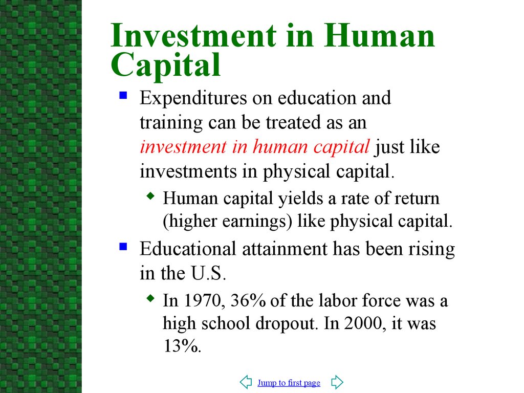
Expenditures on education and
training can be treated as an
investment in human capital just like
investments in physical capital.
Human capital yields a rate of return
(higher earnings) like physical capital.
Educational attainment has been rising
in the U.S.
In 1970, 36% of the labor force was a
high school dropout. In 2000, it was
13%.
Jump to first page
3.
Age-Earnings Profiles, byEducation (1999)
120,000
100,000
Annual Earnings
The male ageearnings
profiles indicate
those with more
education have higher
earnings.
higher
The age-earnings
profiles are steeper
for those with more
education.
Females have flatter
age-earnings profiles.
80,000
60,000
40,000
20,000
0
18-24 25-34 35-44 45-54 55-64
<12
Jump to first page
12
16
17+
65+
4.
Human Capital ModelThe decision should be made by
comparing the costs and benefits
(higher earnings) of college.
Costs of attending college
The direct costs are the cost of tuition,
fees, and books.
Room and board are not included
since they are needed regardless of
whether you go to college.
The indirect cost is the forgone
earnings you give up while you
attending college.
Jump to first page
5.
Age-Earnings With andWithout College
The HH curve is the ageearnings profile if a person
does
not attend college.
The CC curve is the costearnings profile if one
attends college.
The total cost of attending
college is the sum of the
direct costs (area 1) plus
indirect costs (area 2).
The benefit of attending
college is the increase in
earnings due to the college
(areait3).
degree
Whether
is rational to
attend college depends on
whether the
present value
of the benefits exceeds the
present value of the
costs.
Annual Earnings
C
Incremental
Earnings (3)
H
H Indirect
Costs (2)
C
18
22
Jump to first page
65
Direct Costs (1)
Age
6.
Present ValueDiscounting converts the value of
future dollars into today’s dollars
through the interest rate.
The present value (Vp) of a payment
received one year from now is:
Def:
Vp =
Payment 1 year from now
1+Interest rate
where i = 10%
Ex:
Vp = $ 110 = $ 100.00
1.10
Jump to first page
7.
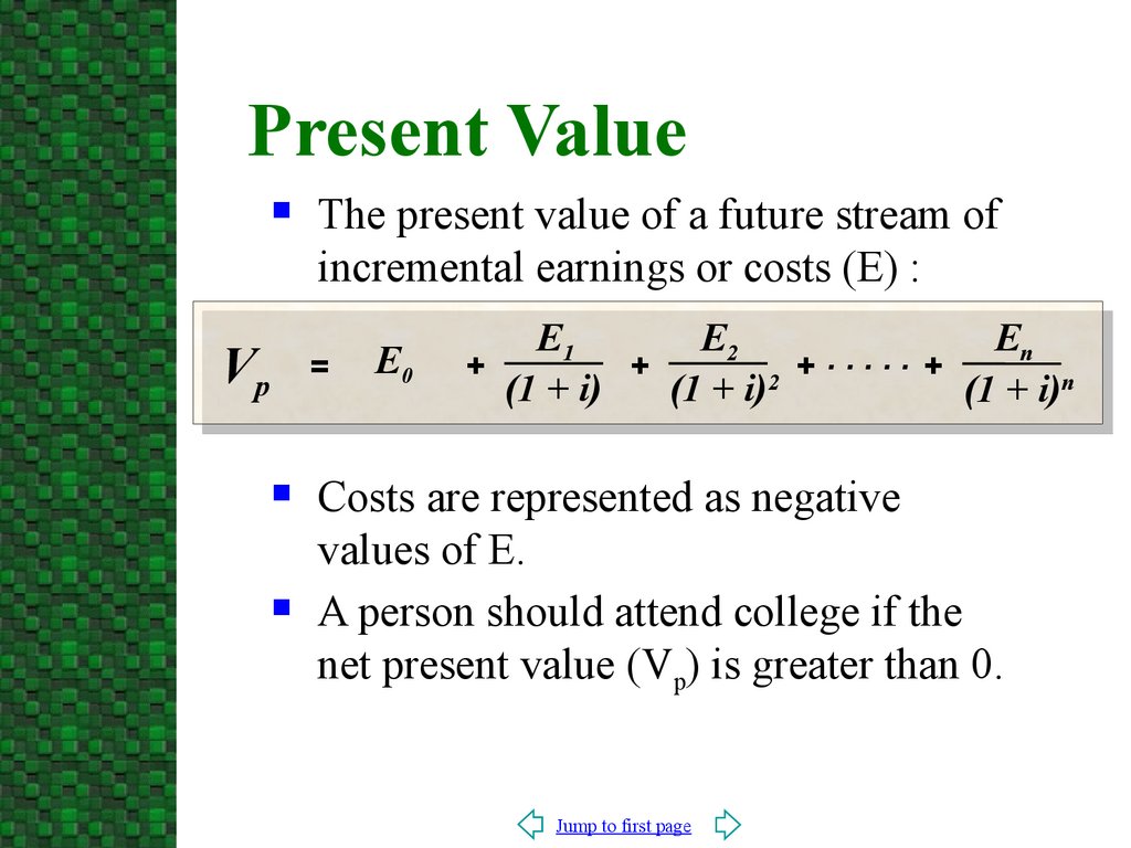
Present ValueVp
The present value of a future stream of
incremental earnings or costs (E) :
=
E0
E1
E2
En
.
.
.
.
.
+
+
+
+
(1 + i)
(1 + i)2
(1 + i)n
Costs are represented as negative
values of E.
A person should attend college if the
net present value (Vp) is greater than 0.
Jump to first page
8.
Discounted Present ValuePV of $8,000 Investment in Webmaster Training Program
(Interest Rate = 10 Percent)
Year
(1)
Incremental
Earnings
(2)
Discounted Value
(10 Percent Rate)
(3)
0
1
2
3
-$ 8,000
$ 3,000
$ 4,000
$ 5,000
1.000
0.909
0.826
0.751
Present Value
of Earnings
(4)
$ -8,000
$ 2,727
$ 3,305
$ 3,755
$ 1,787
Suppose Melinda is considering taking a webmaster training
program that involves direct costs of $3,000 and forgone
earnings
$5,000. The training program will increase
Melinda’s earnings by
$3,000, $4,000, and $5,000 for the 3
she plans
onborrow
working.
years
Because
she can
the funds at an interest rate of 10%, we
will discount the future expected income at an 10% rate.
What is the present value (PV) of this training program?
The PV of the training program is positive, Melinda should take
the training program.
Jump to first page
9.
Internal Rate of ReturnThe internal rate of return, r, is the
rate of return at which Vp = 0:
E1
E2
En
.
.
.
.
.
+
+
+
= 0 = E0 +
(1 + r)
(1 + r)2
(1 + r)n
Vp
A person should attend college if the
rate of return (r) exceeds the market
interest rate (i).
Jump to first page
10.
GeneralizationsLength of income stream
The longer the stream of positive
incremental earnings, the more likely the
net present value will be positive.
As a result, younger people are more
likely to attend college
Costs of attending college
The lower the cost of attending college,
the more likely the net present value is
positive.
Older people have a higher opportunity
cost of attending college, less likely to
attend.
Jump to first page
11.
GeneralizationsEarnings differential
The larger is the college-high school
earnings differential, the more likely the
net present value is greater.
College attendance rose in the 1980s as
the college-high school premium
increased.
Jump to first page
12.
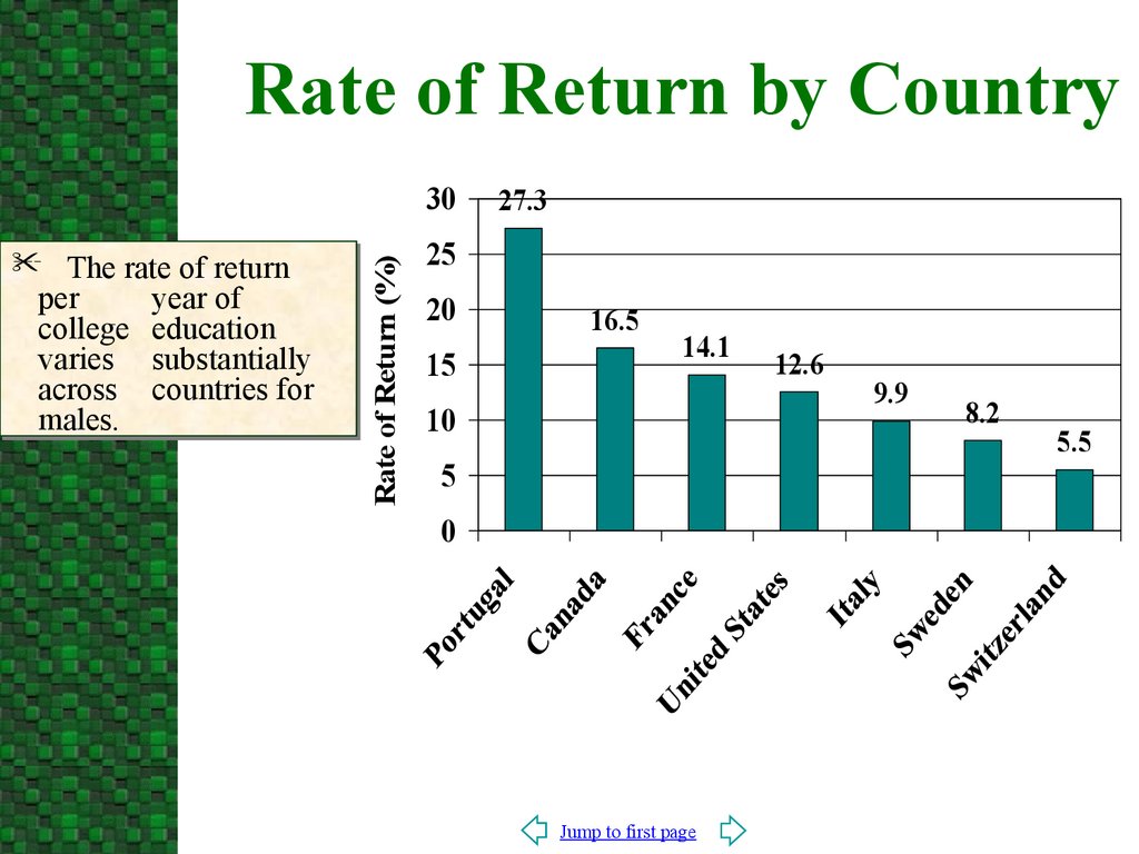
Rate of Return by CountryThe rate of return
per
year of
college education
varies substantially
across countries for
males.
Rate of Return (%)
30
27.3
25
20
15
16.5
14.1
10
5
0
Jump to first page
12.6
9.9
8.2
5.5
13.
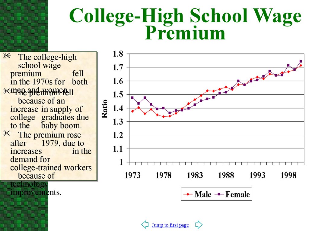
The college-highschool wage
premium
fell
in the 1970s for both
women.
men
The and
premium
fell
because of an
increase in supply of
college graduates due
to the baby boom.
The premium rose
after
1979, due to
increases
in the
demand for
college-trained workers
because of
technology
improvements.
Ratio
College-High School Wage
Premium
1.8
1.7
1.6
1.5
1.4
1.3
1.2
1.1
1
1973
1978
1983
Male
Jump to first page
1988
1993
Female
1998
14.
CaveatsWe can’t predict the college-high school
wage premium for future graduates.
The charts report past differentials
The future differential may be smaller as
the high differential may increase future
supply.
These are average earnings of college and
high school graduates the distribution of
earnings around the mean is wide.
The quality of schooling matters as well
as the quantity of schooling
Jump to first page
15.
Private vs. SocialPerspective
Education yields substantial external or
social benefits that society reaps.
More educated workers have lower
unemployment rates.
Education raises the amount and quality of
participation in the political process.
Children grow up in a better homeenvironment if the parents are more
educated.
The research discoveries of more educated
persons yield benefits to society.
Jump to first page
16.
Private vs. SocialPerspective
The social rate of return is higher (lower)
than the private rate of return, resources
will be underallocated (overallocated) to
human capital investments.
The private and social rate of return are
quite similar.
Jump to first page
17.
3. Human CapitalInvestment and the
Distribution of Earnings
Jump to first page
18.
The marginal rate of return toeducation declines as
additional
schooling is
acquired.
Investment in education is
subject to the law of
diminishing returns. The
increases in knowledge decline
with each additional year of
schooling.
The return also falls because
the
explicit cost and
opportunity
cost of
education rises with
additional schooling.
Rate of Return
Diminishing Rate of
Return
r
Years of Schooling
Jump to first page
19.
Since individuals shouldincrease schooling so that the
marginal
rate of return
of schooling (r) is
equal
the interest
(i).at interest
to Using
the r=irate
rule,
rate i2, the optimal level of
schooling is e2.
At i1 the optimal level is e1.
At i3 the optimal level is e3.
Each equilibrium point (1,2,3)
indicates the “price” and
quantity demanded of human
capital. In other words, the
demand for human capital.
r, i
Demand for Human
Capital
1
i1
S1
2
i2
3
i3
e1
Jump to first page
e2
e3
S2
S3
r, DHC
Years of
Schooling
20.
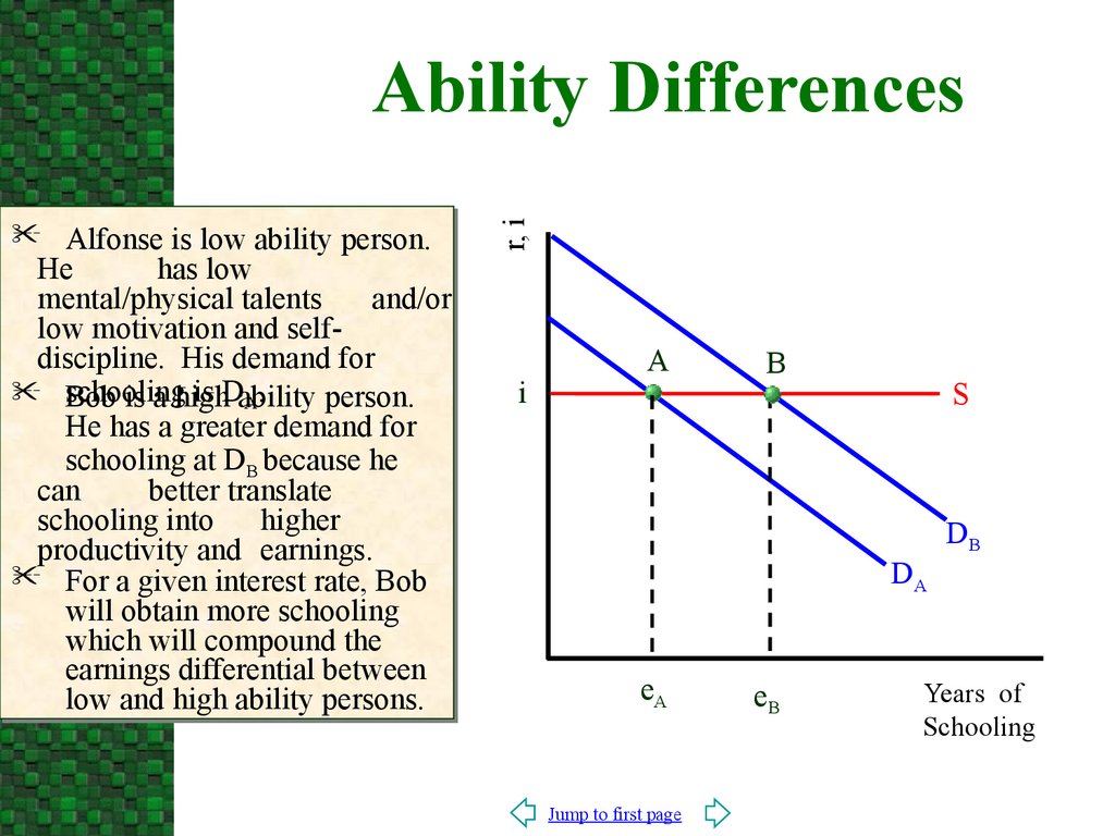
Alfonse is low ability person.He
has low
mental/physical talents
and/or
low motivation and selfdiscipline. His demand for
is Dability
schooling
Bob is a high
person.
A.
He has a greater demand for
schooling at DB because he
can
better translate
schooling into higher
productivity and earnings.
For a given interest rate, Bob
will obtain more schooling
which will compound the
earnings differential between
low and high ability persons.
r, i
Ability Differences
i
A
B
S
DA
eA
Jump to first page
eB
DB
Years of
Schooling
21.
Albert is black and isdiscriminated against in the labor
market. His demand for
schooling is DA since he has low
ability to convert additional
schooling into higher earnings.
Brett is white and has a
greater demand for schooling
at DB as he can reap the
benefits of
additional
schooling.
For a given interest rate, Bret
will obtain more schooling
which will compound the
earnings differential between
whites and blacks.
r, i
Discrimination
i
A
B
S
DA
eA
Jump to first page
eB
DB
Years of
Schooling
22.
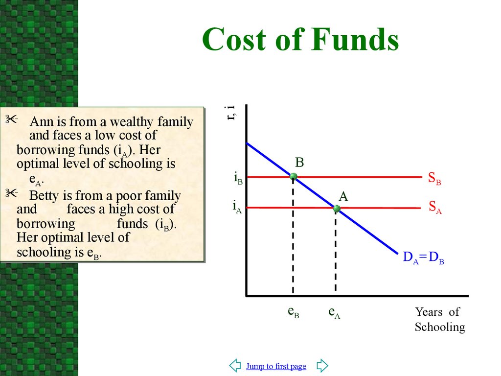
Ann is from a wealthy familyand faces a low cost of
borrowing funds (iA). Her
optimal level of schooling is
eA.
Betty is from a poor family
and
faces a high cost of
borrowing
funds (iB).
Her optimal level of
schooling is eB.
r, i
Cost of Funds
iB
B
A
iA
SB
SA
D A= D B
eB
Jump to first page
eA
Years of
Schooling
23.
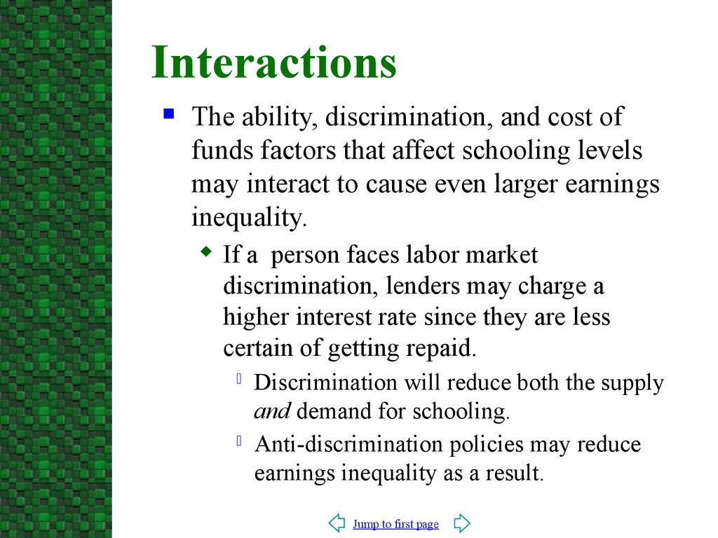
InteractionsThe ability, discrimination, and cost of
funds factors that affect schooling levels
may interact to cause even larger earnings
inequality.
If a person faces labor market
discrimination, lenders may charge a
higher interest rate since they are less
certain of getting repaid.
Discrimination will reduce both the supply
and demand for schooling.
Anti-discrimination policies may reduce
earnings inequality as a result.
Jump to first page
24.
Capital MarketImperfections
The capital market is biased in favor of
physical rather than human capital
Lenders can’t repossess human capital.
Young people, who are most likely to
invest in human capital, don’t have
established credit ratings.
The government may have to intervene by
subsidizing human capital loans in order
to make the returns on physical and
human capital equal.
Jump to first page
25.
4. On-the-Job Training(OJT)
Jump to first page
26.
Costs and BenefitsFirms will invest in on-the-job training if
the present value of the benefits of the
training exceeds the present value of the
costs.
The costs to the firm include:
Direct costs such as classroom instruction
and greater worker supervision.
Indirect costs such as reduced worker
output during training.
The benefit is greater worker productivity.
Jump to first page
27.
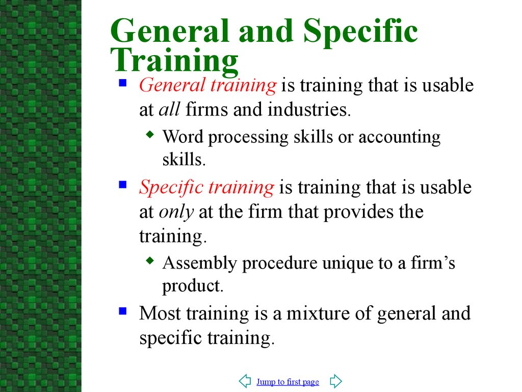
General and SpecificTraining
General training is training that is usable
at all firms and industries.
Word processing skills or accounting
skills.
Specific training is training that is usable
at only at the firm that provides the
training.
Assembly procedure unique to a firm’s
product.
Most training is a mixture of general and
specific training.
Jump to first page
28.
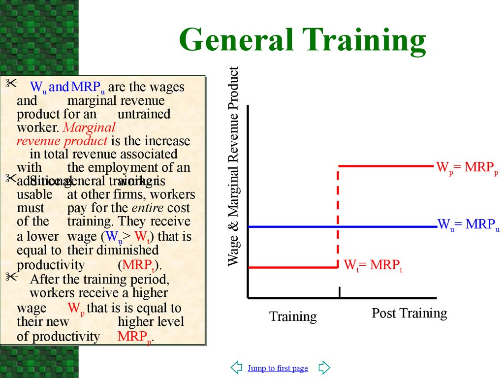
Wu and MRPu are the wagesand
marginal revenue
product for an
untrained
worker. Marginal
revenue product is the increase
in total revenue associated
with
the employment of an
additional
Since general training
worker.is
usable at other firms, workers
must
pay for the entire cost
of the training. They receive
a lower wage (Wu> Wt) that is
equal to their diminished
productivity
(MRPt).
After the training period,
workers receive a higher
wage Wp that is is equal to
their new
higher level
of productivity MRPp.
Wage & Marginal Revenue Product
General Training
Wp= MRPp
Wu= MRPu
Wt= MRPt
Training
Jump to first page
Post Training
29.
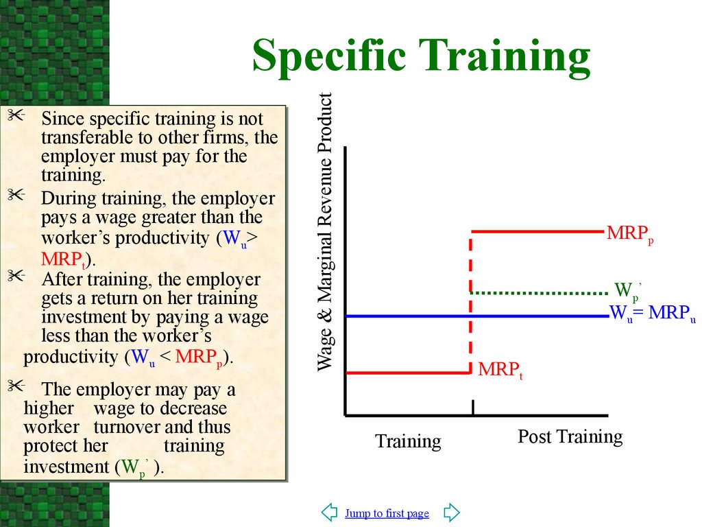
Since specific training is nottransferable to other firms, the
employer must pay for the
training.
During training, the employer
pays a wage greater than the
worker’s productivity (Wu>
MRPt).
After training, the employer
gets a return on her training
investment by paying a wage
less than the worker’s
productivity (Wu < MRPp).
The employer may pay a
higher wage to decrease
worker turnover and thus
protect her
training
investment (Wp’ ).
Wage & Marginal Revenue Product
Specific Training
MRPp
Wp’
Wu= MRPu
MRPt
Training
Jump to first page
Post Training
30.
ModificationsFaced with a minimum wage, some firms
may pay for general training.
The firms recoup their expenses by pay
workers less than their MRP after the
training is completed.
This is possible because workers are not
perfectly mobile across jobs—there are
costs to switching jobs.
Workers with the most formal education
also receive more on-the-job training.
They have shown they can receive
training more readily and thus less cost.
Jump to first page