


 economics
Similar presentations:


")


Principles of Macroeconomics
1.
Principles of MacroeconomicsGlobal Edition
Chapter 3
Demand, Supply, and
Market Equilibrium
Copyright © 2020 Pearson Education Ltd. All Rights Reserved.
2.
Chapter Outline and LearningObjectives (1 of 2)
3.1 Firms and Households: The Basic Decision-Making
Units
• Understand the roles of firms, entrepreneurs, and households
in the market.
3.2 Input Markets and Output Markets: The Circular Flow
• Understand the role of households as both suppliers to firms
and buyers of what firms produce.
3.3 Demand in Product/Output Markets
• Understand what determines the position and shape of the
demand curve and what factors move you along a demand
curve and what factors shift the demand curve.
Copyright © 2020 Pearson Education Ltd. All Rights Reserved.
3.
Chapter Outline and LearningObjectives (2 of 2)
3.4 Supply in Product/Output Markets
• Be able to distinguish between forces that shift a supply
curve and changes that cause a movement along a
supply curve.
3.5 Market Equilibrium
• Be able to explain how a market that is not in equilibrium
responds to restore an equilibrium.
Demand and Supply in Product Markets: A Review
Looking Ahead: Markets and the Allocation of
Resources
Copyright © 2020 Pearson Education Ltd. All Rights Reserved.
4.
Chapter 3 Demand, Supply, andMarket Equilibrium
• Chapter 2 discusses how individuals solve economic
problems directly.
• This chapter explains the basic forces at work in market
systems.
• This chapter explains how individual decisions answer
the three basic economic questions.
Copyright © 2020 Pearson Education Ltd. All Rights Reserved.
5.
Firms and Households: The BasicDecision-Making Units
• firm An organization that transforms resources (inputs)
into products (outputs). Firms are the primary producing
units in a market economy.
• entrepreneur A person who organizes, manages, and
assumes the risks of a firm, taking a new idea or a new
product and turning it into a successful business.
• households The consuming units in an economy.
Copyright © 2020 Pearson Education Ltd. All Rights Reserved.
6.
Input Markets and Output Markets:The Circular Flow (1 of 4)
• product or output markets The markets in which
goods and services are exchanged.
• input or factor markets The markets in which the
resources used to produce goods and services are
exchanged.
Copyright © 2020 Pearson Education Ltd. All Rights Reserved.
7.
Figure 3.1 The Circular Flow ofEconomic Activity
Diagrams like this one show the circular flow of
economic activity, hence the name circular flow
diagram. Here goods and services flow
clockwise: Labor services supplied by
households flow to firms, and goods and
services produced by firms flow to households.
Payment (usually money) flows in the opposite
(counterclockwise) direction: Payment for goods
and services flows from households to firms, and
payment for labor services flows from firms to
households.
Note: Color Guide—In this figure households are
depicted in blue, and firms are depicted in red.
From now on, all diagrams relating to the
behavior of households will be blue or shades of
blue, and all diagrams relating to the behavior of
firms will be red or shades of red. The green
color indicates a monetary flow.
Copyright © 2020 Pearson Education Ltd. All Rights Reserved.
8.
Input Markets and Output Markets:The Circular Flow (2 of 4)
• labor market The input/factor market in which
households supply work for wages to firms that demand
labor.
• capital market The input/factor market in which
households supply their savings, for interest or for claims
to future profits, to firms that demand funds to buy capital
goods.
Copyright © 2020 Pearson Education Ltd. All Rights Reserved.
9.
Input Markets and Output Markets:The Circular Flow (3 of 4)
• land market The input/factor market in which
households supply land or other real property in
exchange for rent.
• factors of production The inputs into the production
process. Land, labor, and capital are the three key
factors of production.
Copyright © 2020 Pearson Education Ltd. All Rights Reserved.
10.
Input Markets and Output Markets:The Circular Flow (4 of 4)
• Input and output markets are connected through the
behavior of both firms and households.
• Firms determine the quantities and character of outputs
produced and the types and quantities of inputs
demanded.
• Households determine the types and quantities of
products demanded and the quantities and types of
inputs supplied.
Copyright © 2020 Pearson Education Ltd. All Rights Reserved.
11.
Demand in Product/Output Markets(1 of 2)
• A household’s decision about what quantity of a particular
output, or product, to demand depends on a number of
factors, including:
– The price of the product in question
– The income available to the household
– The household’s amount of accumulated wealth
– The prices of other products available to the household
– The household’s tastes and preferences
– The household’s expectations about future income,
wealth, and prices
Copyright © 2020 Pearson Education Ltd. All Rights Reserved.
12.
Demand in Product/Output Markets(2 of 2)
• quantity demanded The amount (number of units) of a
product that a household would buy in a given period if it
could buy all it wanted at the current market price.
• It is important to focus on the price change alone with
the ceteris paribus, or “all else equal,” assumption.
Copyright © 2020 Pearson Education Ltd. All Rights Reserved.
13.
Changes in Quantity Demandedversus Changes in Demand
• Changes in the price of a product affect the quantity
demanded per period.
• Changes in any other factor, such as income or
preferences, affect demand.
• Thus, we say that an increase in the price of Coca-Cola
is likely to cause a decrease in the quantity of Coca-Cola
demanded. However, we say that an increase in income
is likely to cause an increase in the demand for most
goods.
Copyright © 2020 Pearson Education Ltd. All Rights Reserved.
14.
Price and Quantity Demanded: TheLaw of Demand (1 of 3)
• demand schedule Shows how much of a given product
a household would be willing to buy at different prices for
a given time period.
• demand curve A graph illustrating how much of a given
product a household would be willing to buy at different
prices.
Copyright © 2020 Pearson Education Ltd. All Rights Reserved.
15.
Table 3.1 Alex’s Demand Schedulefor Gasoline
Price
(per Gallon)
Quantity Demanded
(Gallons per Week)
$8.00
7.00
6.00
5.00
4.00
3.00
2.00
1.00
0.00
0
2
3
5
7
10
14
20
26
Copyright © 2020 Pearson Education Ltd. All Rights Reserved.
16.
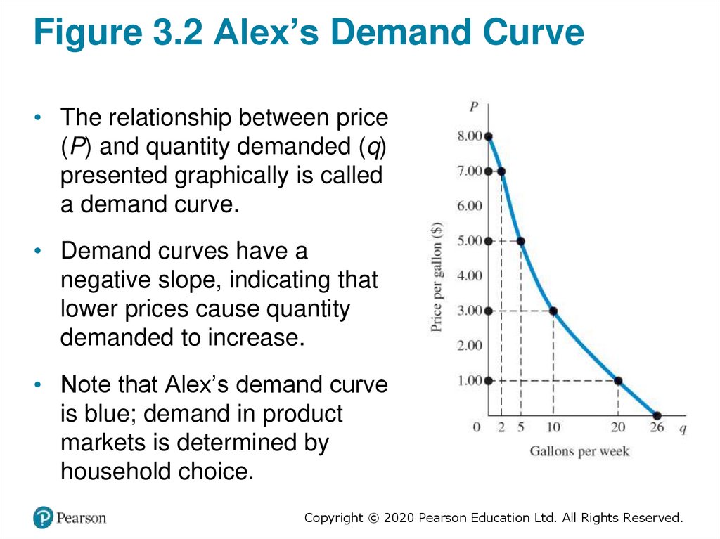
Figure 3.2 Alex’s Demand Curve• The relationship between price
(P) and quantity demanded (q)
presented graphically is called
a demand curve.
• Demand curves have a
negative slope, indicating that
lower prices cause quantity
demanded to increase.
• Note that Alex’s demand curve
is blue; demand in product
markets is determined by
household choice.
Copyright © 2020 Pearson Education Ltd. All Rights Reserved.
17.
Price and Quantity Demanded: TheLaw of Demand (2 of 3)
Demand Curves Slope Downward
• law of demand The negative relationship between price
and quantity demanded: Ceteris paribus, as price rises,
quantity demanded decreases; as price falls, quantity
demanded increases during a given period of time, all
other things remaining constant.
• It is reasonable to expect quantity demanded to fall when
price rises, ceteris paribus, and to expect quantity
demanded to rise when price falls, ceteris paribus.
• A demand curve has a negative slope.
Copyright © 2020 Pearson Education Ltd. All Rights Reserved.
18.
Price and Quantity Demanded: TheLaw of Demand (3 of 3)
Other Properties of Demand Curves
• To summarize what we know about the shape of demand
curves:
1. They have a negative slope.
2. They intersect the quantity (X) axis, a result of time
limitations and diminishing marginal utility.
3. They intersect the price (Y) axis, a result of limited
income and wealth.
• The actual shape of an individual household demand
curve depends on the unique tastes and preferences of
the household and other factors.
Copyright © 2020 Pearson Education Ltd. All Rights Reserved.
19.
Other Determinants of HouseholdDemand (1 of 3)
Income and Wealth
• income The sum of all a household’s wages, salaries,
profits, interest payments, rents, and other forms of
earnings in a given period of time. It is a flow measure.
• wealth or net worth The total value of what a household
owns minus what it owes. It is a stock measure.
Copyright © 2020 Pearson Education Ltd. All Rights Reserved.
20.
Other Determinants of HouseholdDemand (2 of 3)
Income and Wealth
• normal goods Goods for which demand goes up when
income is higher and for which demand goes down when
income is lower.
• inferior goods Goods for which demand tends to fall
when income rises.
Copyright © 2020 Pearson Education Ltd. All Rights Reserved.
21.
Other Determinants of HouseholdDemand (3 of 3)
Prices of Other Goods and Services
• substitutes Goods that can serve as replacements for
one another; when the price of one increases, demand
for the other increases.
• perfect substitutes Identical products.
• complements, complementary goods Goods that “go
together”; a decrease in the price of one results in an
increase in demand for the other and vice versa.
Copyright © 2020 Pearson Education Ltd. All Rights Reserved.
22.
ECONOMICS IN PRACTICE (1 of 4)Have You Bought This Textbook?
One might think that the total number of
textbooks, used plus new, should match class
enrollment. After all, the text is required!
Economists found that the higher the textbook
price, the more text sales fell below class
enrollments.
Students found substitutes when textbook
prices were high.
CRITICAL THINKING
1.
If you were to construct a demand curve for a required text in a course, where would
that demand curve intersect the horizontal axis?
2.
In the year before a new edition of a text is published, many college bookstores will
not buy the older edition. Given this fact, what do you think happens to the gap
between enrollments and new plus used book sales in the year before a new edition
of a text is expected?
Copyright © 2020 Pearson Education Ltd. All Rights Reserved.
23.
Other Determinants of HouseholdDemand ( 1 of 2)
Tastes and Preferences
• Changes in preferences can and do manifest themselves
in market behavior.
• Within the constraints of prices and incomes, preference
shapes the demand curve, but it is difficult to generalize
about tastes and preferences.
Copyright © 2020 Pearson Education Ltd. All Rights Reserved.
24.
ECONOMICS IN PRACTICE (2 of 4)People Drink Tea on Rainy Days
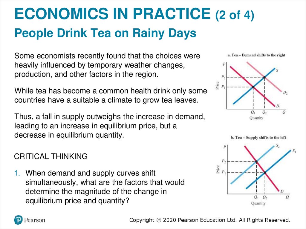
Some economists recently found that the choices were
heavily influenced by temporary weather changes,
production, and other factors in the region.
While tea has become a common health drink only some
countries have a suitable a climate to grow tea leaves.
Thus, a fall in supply outweighs the increase in demand,
leading to an increase in equilibrium price, but a
decrease in equilibrium quantity.
CRITICAL THINKING
1. When demand and supply curves shift
simultaneously, what are the factors that would
determine the magnitude of the change in
equilibrium price and quantity?
Copyright © 2020 Pearson Education Ltd. All Rights Reserved.
25.
Other Determinants of HouseholdDemand (2 of 2)
Expectations
• What you decide to buy today certainly depends on
today’s prices and your current income and wealth.
• Increasingly, economic theory has come to recognize the
importance of expectations.
• It is important to understand that demand depends on
more than just current incomes, prices, and tastes.
Copyright © 2020 Pearson Education Ltd. All Rights Reserved.
26.
Shift of Demand versus Movementalong a Demand Curve (1 of 2)
• shift of a demand curve The change that takes place in a
demand curve corresponding to a new relationship
between quantity demanded of a good and price of that
good. The shift is brought about by a change in the
original conditions.
• movement along a demand curve The change in quantity
demanded brought about by a change in price.
Copyright © 2020 Pearson Education Ltd. All Rights Reserved.
27.
TABLE 3.2 Shift of Alex’s DemandSchedule Resulting from an Increase
in Income
Price
(per Gallon)
Schedule D0
Quantity Demanded
(Gallons per Week at an
Income of $500 per Week)
Schedule D1
Quantity Demanded
(Gallons per Week at an
Income of $700 per Week)
$8.00
0
3
7.00
2
5
6.00
3
7
5.00
5
10
4.00
7
12
3.00
10
15
2.00
14
19
1.00
20
24
0.00
26
30
Copyright © 2020 Pearson Education Ltd. All Rights Reserved.
28.
Figure 3.3 Shift of a Demand CurveFollowing a Rise in Income
• When the price of a good
changes, we move along the
demand curve for that good.
• When any other factor that
influences demand changes
(income, tastes, and so on),
the demand curve shifts, in
this case from D0 to D1.
• Gasoline is a normal good,
so an income increase shifts
the curve to the right.
Copyright © 2020 Pearson Education Ltd. All Rights Reserved.
29.
Shift of Demand versus Movementalong a Demand Curve (2 of 2)
• Change in price of a good or service leads to change in
quantity demanded (movement along a demand
curve).
• Change in income, preferences, or prices of other goods
or services leads to change in demand (shift of a
demand curve).
Copyright © 2020 Pearson Education Ltd. All Rights Reserved.
30.
Figure 3.4 Shifts versus Movementalong a Demand Curve (1 of 2)
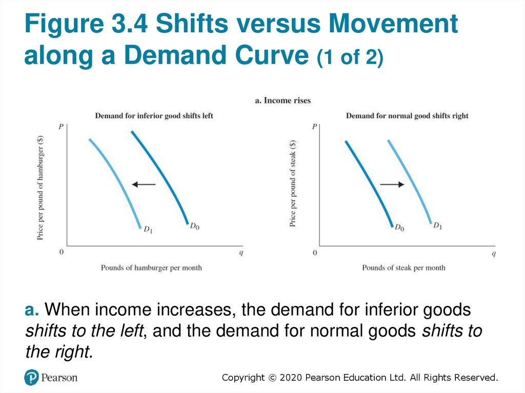
a. When income increases, the demand for inferior goods
shifts to the left, and the demand for normal goods shifts to
the right.
Copyright © 2020 Pearson Education Ltd. All Rights Reserved.
31.
Figure 3.4 Shifts versus Movementalong a Demand Curve (2 of 2)
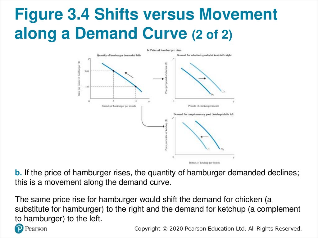
b. If the price of hamburger rises, the quantity of hamburger demanded declines;
this is a movement along the demand curve.
The same price rise for hamburger would shift the demand for chicken (a
substitute for hamburger) to the right and the demand for ketchup (a complement
to hamburger) to the left.
Copyright © 2020 Pearson Education Ltd. All Rights Reserved.
32.
From Household Demand to MarketDemand
• market demand The sum of all the quantities of a good
or service demanded per period by all the households
buying in the market for that good or service.
Copyright © 2020 Pearson Education Ltd. All Rights Reserved.
33.
Figure 3.5 Deriving Market Demandfrom Individual Demand Curves
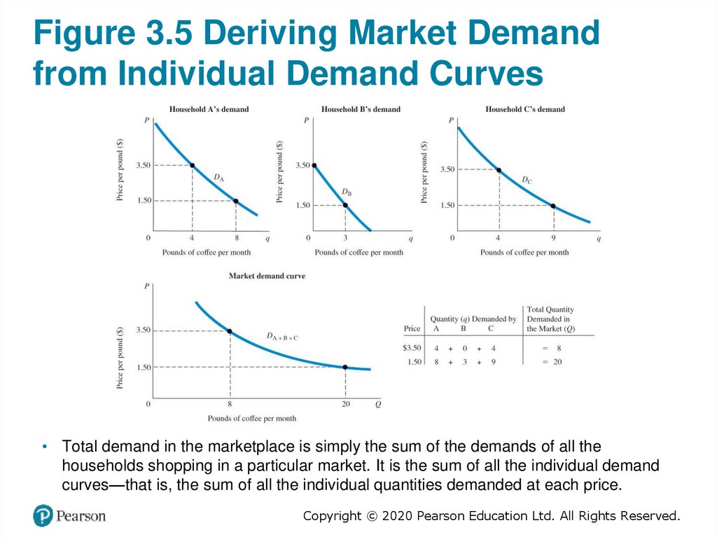
• Total demand in the marketplace is simply the sum of the demands of all the
households shopping in a particular market. It is the sum of all the individual demand
curves—that is, the sum of all the individual quantities demanded at each price.
Copyright © 2020 Pearson Education Ltd. All Rights Reserved.
34.
Supply in Product/Output Markets• Firms build factories, hire workers, and buy raw materials
because they believe they can sell the products they
make for more than it costs to produce them.
• profit The difference between revenues and costs.
Copyright © 2020 Pearson Education Ltd. All Rights Reserved.
35.
Price and Quantity Supplied: TheLaw of Supply (1 of 3)
• quantity supplied The amount of a particular product
that a firm would be willing and able to offer for sale at a
particular price during a given time period.
• supply schedule Shows how much of a product firms
will sell at alternative prices.
Copyright © 2020 Pearson Education Ltd. All Rights Reserved.
36.
Price and Quantity Supplied: TheLaw of Supply (2 of 3)
• law of supply The positive relationship between price
and quantity of a good supplied: An increase in market
price, ceteris paribus, will lead to an increase in quantity
supplied, and a decrease in market price will lead to a
decrease in quantity supplied.
• supply curve A graph illustrating how much of a product
a firm will sell at different prices.
Copyright © 2020 Pearson Education Ltd. All Rights Reserved.
37.
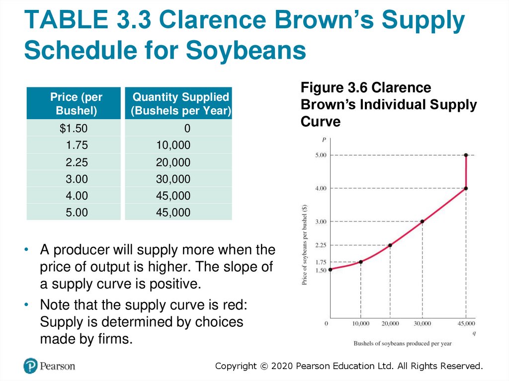
TABLE 3.3 Clarence Brown’s SupplySchedule for Soybeans
Price (per
Bushel)
Quantity Supplied
(Bushels per Year)
$1.50
1.75
0
10,000
2.25
3.00
4.00
5.00
20,000
30,000
45,000
45,000
Figure 3.6 Clarence
Brown’s Individual Supply
Curve
• A producer will supply more when the
price of output is higher. The slope of
a supply curve is positive.
• Note that the supply curve is red:
Supply is determined by choices
made by firms.
Copyright © 2020 Pearson Education Ltd. All Rights Reserved.
38.
Other Determinants of Supply (1 of 2)The Cost of Production
• For a firm to make a profit, its revenue must exceed its
costs.
• Cost of production depends on a number of factors,
including the available technologies and the prices and
quantities of the inputs needed by the firm (labor, land,
capital, energy, and so on).
Copyright © 2020 Pearson Education Ltd. All Rights Reserved.
39.
Other Determinants of Supply (2 of 2)The Prices of Related Products
• Assuming that its objective is to maximize profits, a firm’s
decision to supply depends on:
1. The price of the good or service.
2. The cost of producing the product, which in turn
depends on:
▪ The price of required inputs (labor, capital, and
land)
▪ The technologies that can be used to produce the
product.
3. The prices of related products.
Copyright © 2020 Pearson Education Ltd. All Rights Reserved.
40.
Shift of Supply versus Movementalong a Supply Curve (1 of 2)
• movement along a supply curve The change in
quantity supplied brought about by a change in price.
• shift of a supply curve The change that takes place in a
supply curve corresponding to a new relationship
between quantity supplied of a good and the price of that
good. The shift is brought about by a change in the
original conditions.
Copyright © 2020 Pearson Education Ltd. All Rights Reserved.
41.
TABLE 3.4 Shift of Supply Schedule forSoybeans following Development of a
New Disease-Resistant Seed Strain
Price
(per
Bushel)
$1.50
1.75
Schedule S0
Quantity Supplied
(Bushels per Year
Using Old Seed)
0
10,000
Schedule S1
Quantity Supplied
(Bushels per Year
Using New Seed)
5,000
23,000
2.25
3.00
4.00
20,000
30,000
45,000
33,000
40,000
54,000
Copyright © 2020 Pearson Education Ltd. All Rights Reserved.
42.
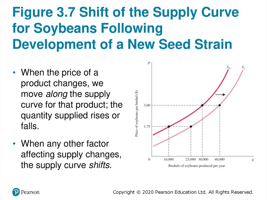
Figure 3.7 Shift of the Supply Curvefor Soybeans Following
Development of a New Seed Strain
• When the price of a
product changes, we
move along the supply
curve for that product; the
quantity supplied rises or
falls.
• When any other factor
affecting supply changes,
the supply curve shifts.
Copyright © 2020 Pearson Education Ltd. All Rights Reserved.
43.
Shift of Supply versus Movementalong a Supply Curve (2 of 2)
• It is very important to distinguish between movements
along supply curves (changes in quantity supplied) and
shifts in supply curves (changes in supply):
• Change in price of a good or service leads to change in
quantity supplied (movement along a supply curve).
• Change in costs, input prices, technology, or prices of
related goods and services leads to change in supply
(shift of a supply curve).
Copyright © 2020 Pearson Education Ltd. All Rights Reserved.
44.
From Individual Supply to MarketSupply
• market supply The sum of all that is supplied each
period by all producers of a single product.
Copyright © 2020 Pearson Education Ltd. All Rights Reserved.
45.
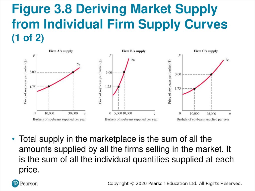
Figure 3.8 Deriving Market Supplyfrom Individual Firm Supply Curves
(1 of 2)
• Total supply in the marketplace is the sum of all the
amounts supplied by all the firms selling in the market. It
is the sum of all the individual quantities supplied at each
price.
Copyright © 2020 Pearson Education Ltd. All Rights Reserved.
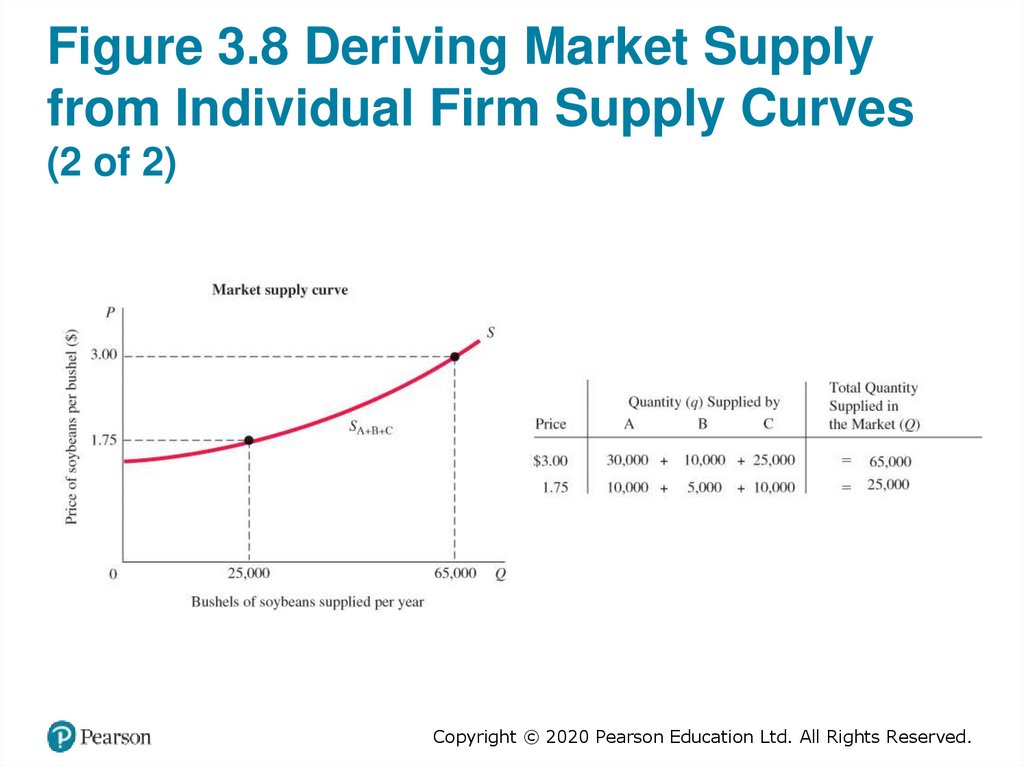
46.
Figure 3.8 Deriving Market Supplyfrom Individual Firm Supply Curves
(2 of 2)
Copyright © 2020 Pearson Education Ltd. All Rights Reserved.
47.
Market Equilibrium• equilibrium The condition that exists when quantity
supplied and quantity demanded are equal. At
equilibrium, there is no tendency for price to change.
Excess Demand
• excess demand or shortage The condition that exists
when quantity demanded exceeds quantity supplied at
the current price.
Copyright © 2020 Pearson Education Ltd. All Rights Reserved.
48.
Figure 3.9 Excess Demand, orShortage
• At a price of $1.75 per bushel, quantity demanded exceeds quantity supplied.
• When excess demand exists, there is a tendency for price to rise.
• When quantity demanded equals quantity supplied, excess demand is eliminated and
the market is in equilibrium.
• Here the equilibrium price is $2.00, and the equilibrium quantity is 40,000 bushels.
Copyright © 2020 Pearson Education Ltd. All Rights Reserved.
49.
Excess Supply• excess supply or surplus The condition that exists
when quantity supplied exceeds quantity demanded at
the current price.
• When quantity supplied exceeds quantity demanded at
the current price, the price tends to fall.
• When price falls, quantity supplied is likely to decrease,
and quantity demanded is likely to increase until an
equilibrium price is reached where quantity supplied and
quantity demanded are equal.
Copyright © 2020 Pearson Education Ltd. All Rights Reserved.
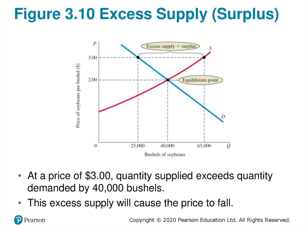
50.
Figure 3.10 Excess Supply (Surplus)• At a price of $3.00, quantity supplied exceeds quantity
demanded by 40,000 bushels.
• This excess supply will cause the price to fall.
Copyright © 2020 Pearson Education Ltd. All Rights Reserved.
51.
Market Equilibrium with Equations (1 of 3)• When economists work with demand and supply, they use
equations to measure the quantitative size of markets.
• Assume demand is a straight (linear) line, then the equation of
the inverse demand curve is
P a - bQd
where Qd = quantity demanded in units
P = price
a = y intercept (price at which quantity demanded is 0)
b = slope of the demand curve
• The demand curve becomes
Qd a / b - 1/ b P
Copyright © 2020 Pearson Education Ltd. All Rights Reserved.
52.
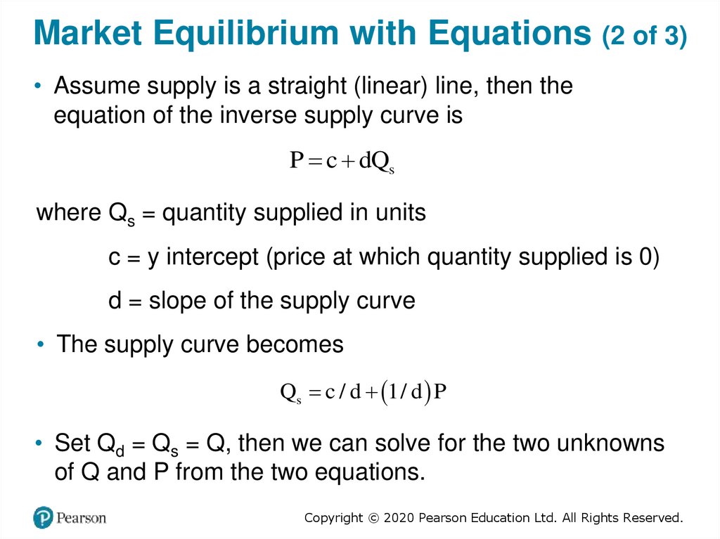
Market Equilibrium with Equations (2 of 3)• Assume supply is a straight (linear) line, then the
equation of the inverse supply curve is
P c dQs
where Qs = quantity supplied in units
c = y intercept (price at which quantity supplied is 0)
d = slope of the supply curve
• The supply curve becomes
Qs c / d 1/ d P
• Set Qd = Qs = Q, then we can solve for the two unknowns
of Q and P from the two equations.
Copyright © 2020 Pearson Education Ltd. All Rights Reserved.
53.
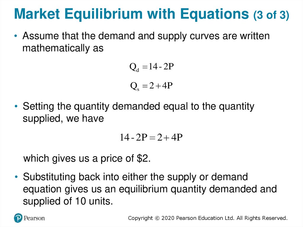
Market Equilibrium with Equations (3 of 3)• Assume that the demand and supply curves are written
mathematically as
Qd 14 - 2P
Qs 2 4P
• Setting the quantity demanded equal to the quantity
supplied, we have
14 - 2P 2 4P
which gives us a price of $2.
• Substituting back into either the supply or demand
equation gives us an equilibrium quantity demanded and
supplied of 10 units.
Copyright © 2020 Pearson Education Ltd. All Rights Reserved.
54.
Changes in Equilibrium• When supply and demand curves shift, the equilibrium
price and quantity change.
Copyright © 2020 Pearson Education Ltd. All Rights Reserved.
55.
Figure 3.11 The Coffee Market: AShift of Supply and Subsequent
Price Adjustment
• Before the freeze, the coffee
market was in equilibrium at
a price of $1.20 per pound.
• At that price, quantity
demanded equaled quantity
supplied.
• The freeze shifted the
supply curve to the left (from
S0 to S1), increasing the
equilibrium price to $2.40.
Copyright © 2020 Pearson Education Ltd. All Rights Reserved.
56.
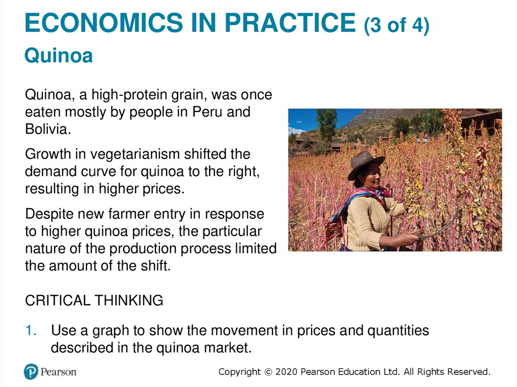
ECONOMICS IN PRACTICE (3 of 4)Quinoa
Quinoa, a high-protein grain, was once
eaten mostly by people in Peru and
Bolivia.
Growth in vegetarianism shifted the
demand curve for quinoa to the right,
resulting in higher prices.
Despite new farmer entry in response
to higher quinoa prices, the particular
nature of the production process limited
the amount of the shift.
CRITICAL THINKING
1. Use a graph to show the movement in prices and quantities
described in the quinoa market.
Copyright © 2020 Pearson Education Ltd. All Rights Reserved.
57.
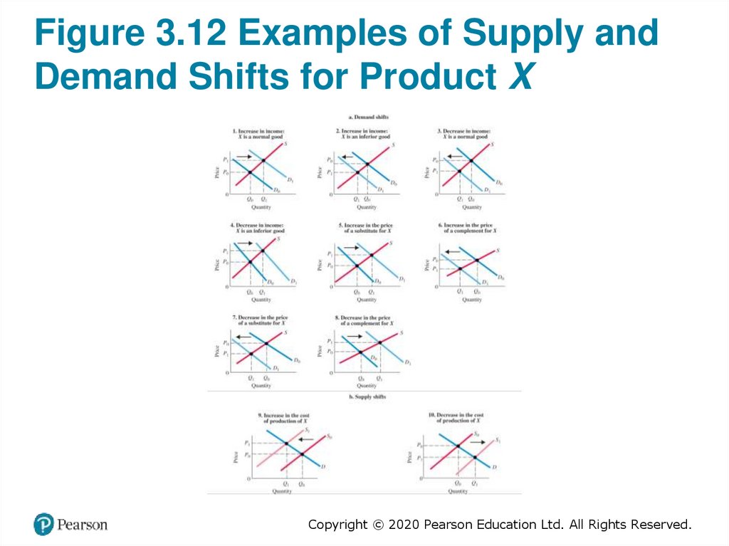
Figure 3.12 Examples of Supply andDemand Shifts for Product X
Copyright © 2020 Pearson Education Ltd. All Rights Reserved.
58.
Demand and Supply in ProductMarkets: A Review (1 of 2)
• Important points to remember about the mechanics of supply and
demand in product markets:
1. A demand curve shows how much of a product a household
would buy if it could buy all it wanted at the given price. A
supply curve shows how much of a product a firm would supply
if it could sell all it wanted at the given price.
2. Demand and supply can also be represented by equations.
3. Quantity demanded and quantity supplied are always per time
period—that is, per day, per month, or per year.
4. The demand for a good is determined by price, household
income and wealth, prices of other goods and services, tastes
and preferences, and expectations.
Copyright © 2020 Pearson Education Ltd. All Rights Reserved.
59.
Demand and Supply in ProductMarkets: A Review (2 of 2)
5. The supply of a good is determined by price, costs of
production, and prices of related products. Costs of
production are determined by available technologies of
production and input prices.
6. Be careful to distinguish between movements along
supply and demand curves and shifts of these curves.
When the price of a good changes, the quantity of that
good demanded or supplied changes—that is, a
movement occurs along the curve. When any other
factor changes, the curve shifts, or changes position.
7. Market equilibrium exists only when quantity supplied
equals quantity demanded at the current price.
Copyright © 2020 Pearson Education Ltd. All Rights Reserved.
60.
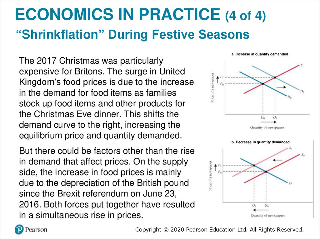
ECONOMICS IN PRACTICE (4 of 4)“Shrinkflation” During Festive Seasons
a. Increase in quantity demanded
The 2017 Christmas was particularly
expensive for Britons. The surge in United
Kingdom’s food prices is due to the increase
in the demand for food items as families
stock up food items and other products for
the Christmas Eve dinner. This shifts the
demand curve to the right, increasing the
equilibrium price and quantity demanded.
b. Decrease in quantity demanded
But there could be factors other than the rise
in demand that affect prices. On the supply
side, the increase in food prices is mainly
due to the depreciation of the British pound
since the Brexit referendum on June 23,
2016. Both forces put together have resulted
in a simultaneous rise in prices.
Copyright © 2020 Pearson Education Ltd. All Rights Reserved.
61.
Looking Ahead: Markets and theAllocation of Resources
You can see how markets answer the basic economic questions
of what is produced, how it is produced, and who gets what is
produced:
• Demand curves reflect what people are willing and able to pay
for products; they are influenced by incomes, wealth,
preferences, prices of other goods, and expectations.
• Firms in business to make a profit have a good reason to
choose the best available technology—lower costs mean
higher profits.
• When a good is in short supply, price rises. As it does, only
those who are willing and able to continue buying do so.
Copyright © 2020 Pearson Education Ltd. All Rights Reserved.
62.
Review Terms and Concepts (1 of 2)• capital market
• firm
• complements, complementary • households
goods
• income
• demand curve
• inferior goods
• demand schedule
• input or factor markets
• entrepreneur
• labor market
• equilibrium
• land market
• excess demand or shortage
• law of demand
• excess supply or surplus
• law of supply
• factors of production
Copyright © 2020 Pearson Education Ltd. All Rights Reserved.
63.
Review Terms and Concepts (2 of 2)• market demand
• quantity demanded
• market supply
• quantity supplied
• movement along a demand
curve
• shift of a demand curve
• movement along a supply
curve
• shift of a supply curve
• substitutes
• supply curve
• normal goods
• supply schedule
• perfect substitutes
• product or output markets
• wealth or net worth
• profit
Copyright © 2020 Pearson Education Ltd. All Rights Reserved.
64.
CopyrightThis work is protected by United States copyright laws and is
provided solely for the use of instructors in teaching their
courses and assessing student learning. Dissemination or sale of
any part of this work (including on the World Wide Web) will
destroy the integrity of the work and is not permitted. The work
and materials from it should never be made available to students
except by instructors using the accompanying text in their
classes. All recipients of this work are expected to abide by these
restrictions and to honor the intended pedagogical purposes and
the needs of other instructors who rely on these materials.
Copyright © 2020 Pearson Education Ltd. All Rights Reserved.