Компьютерные технологии в атомной отрасли (лекция 6)

1.

Компьютерные технологии в атомной отрасли
Цели курса:
Знакомство с алгоритмами численного моделирования физических процессов
Формирование навыков программирования на Фортране
Приобретение опыта написания научных отчетов
Технологии обучения:
Решение N задач на численное моделирование в процессе обучения
(N – отчетов)
Численное решение тестовой задачи численным методом на экзамене
Лекция 7 – Уравнение переноса нейтронов
(численное решение)

2.

Task 1. Функции, производные и интеграл (численные методы)
Task 2. Моделирование движения тела в поле сил тяжести
Task 3. Решение задачи Коши на примере уравнения
изотопной кинетики
Task 4. Вычисление групповых сечений
Task 5. Метод дискретных ординат в плоской геометрии

3.

Основные темы:
Тема 1. Физические величины в нейтронной физике
Тема 2. Подходы к определению характеристик нейтронного поля
Тема 3. Газокинетическое уравнение переноса нейтронов
Тема 4. Стационарные и нестационарные задачи
Тема 5. Групповой подход (задание 4)
Тема 6. Метод дискретных ординат в плоской геометрии (задание 5)

4.

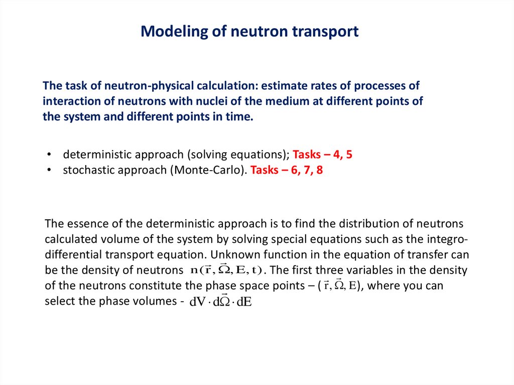
Modeling of neutron transport
The task of neutron-physical calculation: estimate rates of processes of
interaction of neutrons with nuclei of the medium at different points of
the system and different points in time.
• deterministic approach (solving equations); Tasks – 4, 5
• stochastic approach (Monte-Carlo). Tasks – 6, 7, 8
The essence of the deterministic approach is to find the distribution of neutrons
calculated volume of the system by solving special equations such as the integrodifferential transport equation. Unknown
function in the equation of transfer can
be the density of neutrons n ( r , , E, t ) . The first three
variables in the density
of the neutrons constitute the phase
space points – ( r , , E ), where you can
select the phase volumes - dV d dE

5.

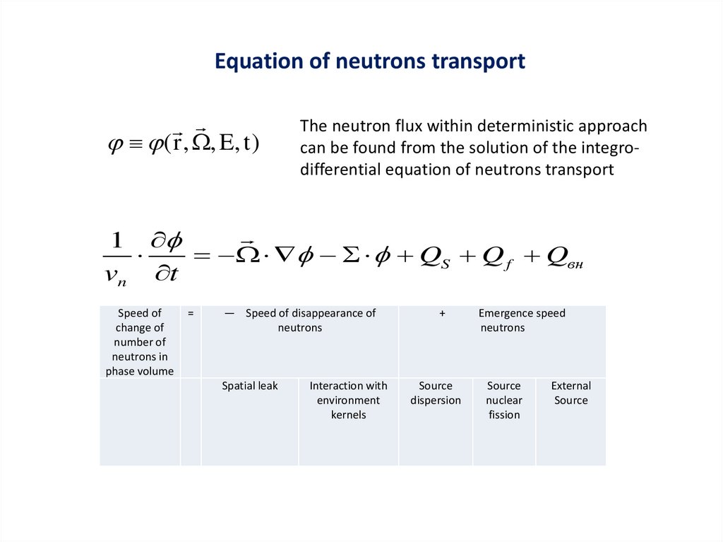
Equation of neutrons transport
( r , , E, t )
The neutron flux within deterministic approach
can be found from the solution of the integrodifferential equation of neutrons transport
1
QS Q f Qвн
vn t
Speed of
change of
number of
neutrons in
phase volume
=
— Speed of disappearance of
neutrons
Spatial leak
Interaction with
environment
kernels
+
Source
dispersion
Emergence speed
neutrons
Source
nuclear
fission
External
Source

6.

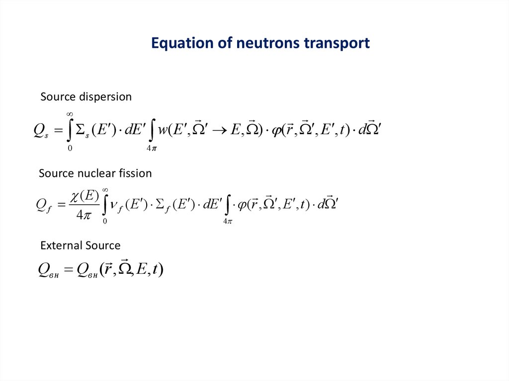
Equation of neutrons transport
Source dispersion
Qs s ( E ) dE w( E , E, ) (r , , E , t ) d
0
4
Source nuclear fission
(E)
Qf
f ( E ) f ( E ) dE (r , , E , t ) d
4 0
4
External Source
Qвн Qвн (r , , E, t )

7.

Scheme of simplification of the equation of neutron transport
Unknown function
( r , , E , t )
Transformation algorithm
Note
It is a lot of variables
Stationary case
( r , , E)
For non-stationary tasks other equations are
solved:
- equation of point kinetics;
- burning out equations (isotope kinetics).
Group approach
(G of power groups)
G equations
Formation of library of group constants
(Task 4)
Sampling of an angular variable
(M of the allocated directions)
G*M equations (Task 5)
Choice of quadratures.
Also, transition to diffusive approach is
possible
g ( r , )
mg ( r )
Internal iterations
Sampling of a spatial variable
(K of spatial cells)
G*M*K of the equations (Task 5)
mg,k
External iterations
Spatial grid.
Volumes and surfaces of cells.

8.

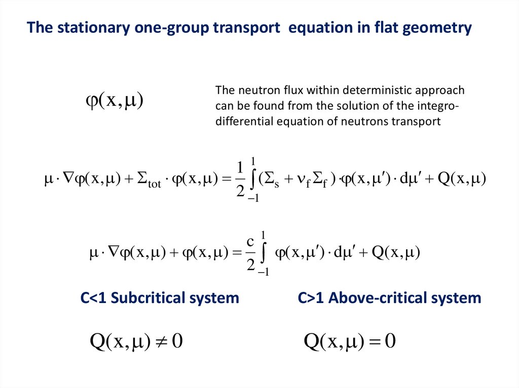
The stationary one-group transport equation in flat geometry
( x, )
The neutron flux within deterministic approach
can be found from the solution of the integrodifferential equation of neutrons transport
11
( x, ) tot ( x, ) ( s f f ) ( x, ) d Q( x, )
2 1
c1
( x, ) ( x, ) ( x, ) d Q( x, )
2 1
C<1 Subcritical system
Q( x, ) 0
C>1 Above-critical system
Q(x, ) 0

9.

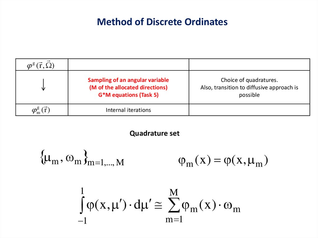
Method of Discrete Ordinates
( r , )
g
Sampling of an angular variable
(M of the allocated directions)
G*M equations (Task 5)
mg ( r )
Choice of quadratures.
Also, transition to diffusive approach is
possible
Internal iterations
Quadrature set
m , m m 1,..., M
m ( x ) ( x, m )
1
M
1
m 1
( x, ) d m ( x ) m

10.

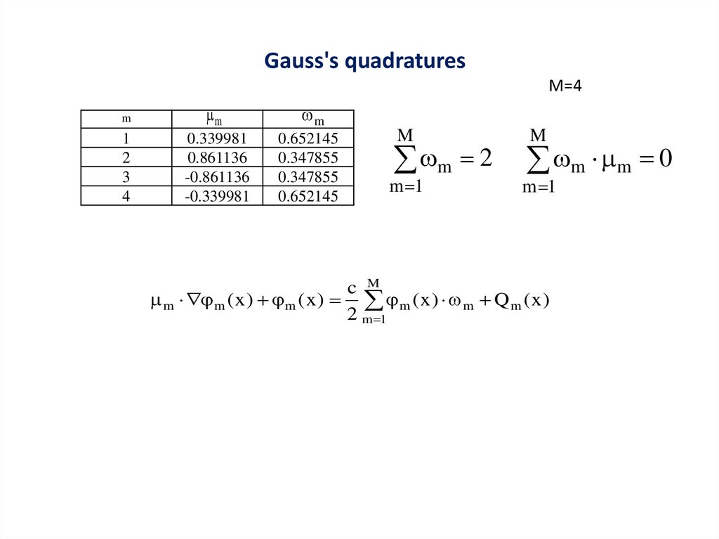
Gauss's quadratures
M=4
m
m
m
1
2
3
4
0.339981
0.861136
-0.861136
-0.339981
0.652145
0.347855
0.347855
0.652145
M
m 2
m 1
M
m m 0
m 1
c M
m m ( x ) m ( x ) m ( x ) m Q m ( x )
2 m 1

11.

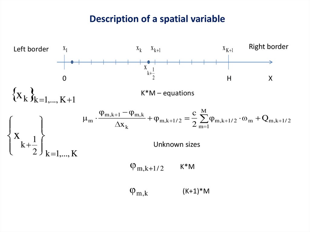
Description of a spatial variable
Left border
x1
xk
x k 1
x
0
x k k 1,..., K 1
x 1
k 2 k 1,..., K
k
1
2
x K 1
Right border
Н
X
K*M – equations
m
m,k 1 m,k
x k
m,k 1 / 2
c M
m,k 1 / 2 m Q m,k 1 / 2
2 m 1
Unknown sizes
m ,k 1 / 2
m ,k
K*M
(K+1)*M

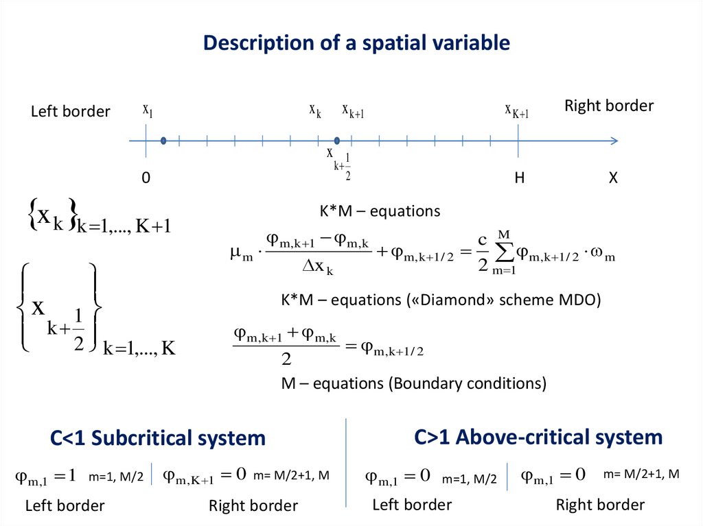
12.

Description of a spatial variable
Left border
x1
xk
x k 1
x
0
x k k 1,..., K 1
x 1
k 2 k 1,..., K
m=1, M/2
Left border
1
2
Right border
Н
X
K*M – equations
m,k 1 m,k
c M
m
m,k 1 / 2 m,k 1 / 2 m
x k
2 m 1
K*M – equations («Diamond» scheme MDO)
m,k 1 m,k
m,k 1 / 2
2
M – equations (Boundary conditions)
C<1 Subcritical system
m,1 1
k
x K 1
m ,K 1 0
m= M/2+1, M
Right border
C>1 Above-critical system
m ,1 0
m=1, M/2
Left border
m ,1 0
m= M/2+1, M
Right border

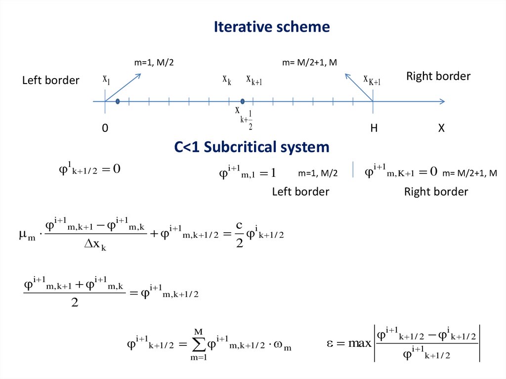
13.

Iterative scheme
m=1, M/2
Left border
m= M/2+1, M
x1
xk
x k 1
x
0
k
1
2
x K 1
Right border
Н
X
C<1 Subcritical system
1k 1 / 2 0
m=1, M/2
i 1m ,1 1
Left border
i 1m,K 1 0
m= M/2+1, M
Right border
i 1m,k 1 i 1m,k
c
m
i 1m,k 1 / 2 i k 1 / 2
x k
2
i 1m,k 1 i 1m,k
i 1m,k 1 / 2
2
i 1k 1 / 2
M
i 1m,k 1 / 2
m 1
m
i 1k 1 / 2 i k 1 / 2
max
i 1k 1 / 2

14.

Iterative scheme
m=1, M/2
m= M/2+1, M
x1
Left border
xk
x k 1
x
0
k
1
2
x K 1
Right border
Н
X
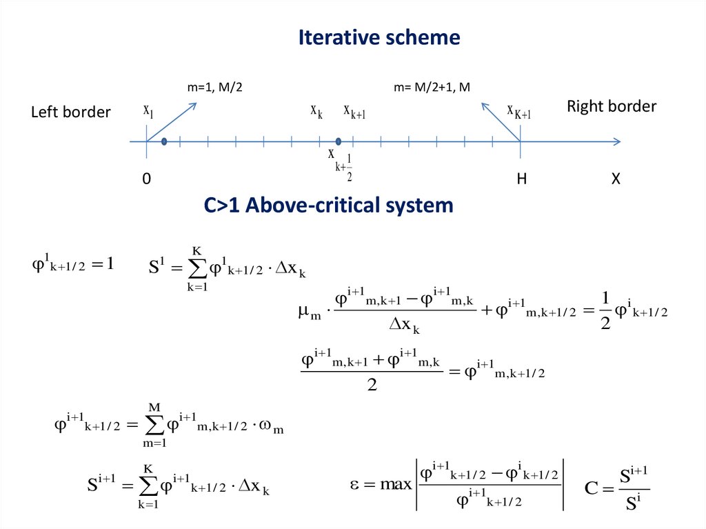
C>1 Above-critical system
1k 1 / 2 1
K
S 1k 1 / 2 x k
1
k 1
i 1m,k 1 i 1m,k
1
m
i 1m,k 1 / 2 i k 1 / 2
x k
2
i 1m,k 1 i 1m,k
i 1m,k 1 / 2
2
i 1k 1 / 2
M
i 1m,k 1 / 2 m
m 1
i 1
S
K
k 1
i 1k 1 / 2
x k
i 1k 1 / 2 i k 1 / 2
max
i 1k 1 / 2
Si 1
C i
S

15.

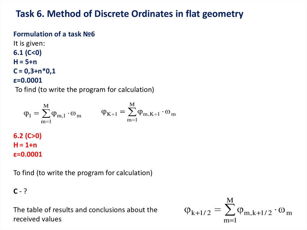
Task 6. Method of Discrete Ordinates in flat geometry
Formulation of a task №6
It is given:
6.1 (C<0)
H = 5+n
C = 0,3+n*0,1
ε=0.0001
To find (to write the program for calculation)
1
M
m,1 m
m 1
K 1
M
m,K 1 m
m 1
6.2 (C>0)
H = 1+n
ε=0.0001
To find (to write the program for calculation)
C-?
The table of results and conclusions about the
received values
k 1 / 2
M
m,k 1 / 2 m
m 1