Research methodology

1.

RESEARCH METHODOLOGY
Olga Konnikova
Ass.Prof. of Marketing Department, Saint-Petersburg State University of Economics
PhD in Economics
E-mail: [email protected]

2.

AGENDA
1.
Quantitative research in Management: methodology. Introduction to IBM SPSS – September 6
2.
Data visualization. Descriptive statistics. Cross-tabulating (Contingency tables) – September
13, October 11
3.
Analysis of variance (dispersion analysis)
4.
Correlation and regression analysis
5.
Cluster analysis
6.
Summary
2

3.

DESCRIBING DATA: «FIRST SIGHT ON THE DATA»
Graphical description
E.g., histograms (to identify outlines – «выбросы»)
Numerical descriptive measures
Median, mode
Range, Minimum, Maximum
Mean, Standard deviation
…
3

4.

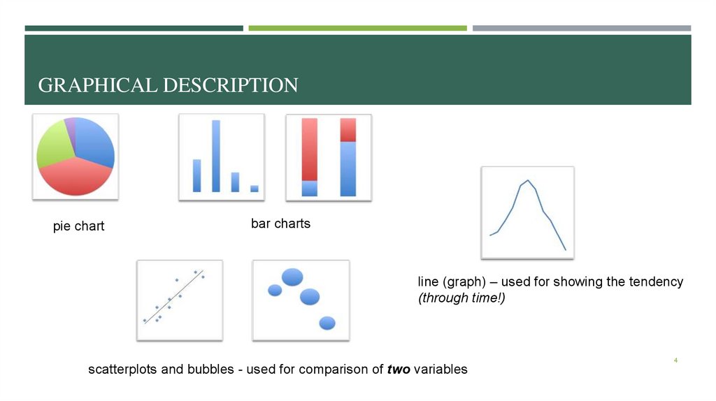
GRAPHICAL DESCRIPTION
pie chart
bar charts
line (graph) – used for showing the tendency
(through time!)
4
scatterplots and bubbles - used for comparison of two variables

5.

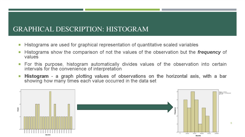
GRAPHICAL DESCRIPTION: HISTOGRAM
Histograms are used for graphical representation of quantitative scaled variables
Histograms show the comparison of not the values of the observation but the frequency of
values
For this purpose, histogram automatically divides values of the observation into certain
intervals for the convenience of interpretation
Histogram - a graph plotting values of observations on the horizontal axis, with a bar
showing how many times each value occurred in the data set
5

6.

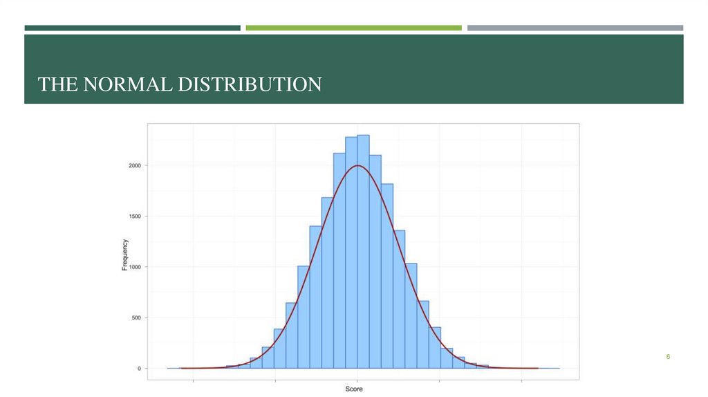
THE NORMAL DISTRIBUTION
6

7.

GRAPHICAL DESCRIPTION: HISTOGRAMS AND NORMAL DISTRIBUTION
The ‘Normal’ distribution
Bell («колокол») shaped
Symmetrical around the center
No outlnine cases
7

8.

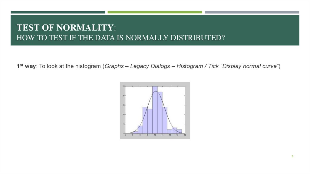
TEST OF NORMALITY:
HOW TO TEST IF THE DATA IS NORMALLY DISTRIBUTED?
1st way: To look at the histogram (Graphs – Legacy Dialogs – Histogram / Tick “Display normal curve”)
8

9.

TEST OF NORMALITY:
HOW TO TEST IF THE DATA IS NORMALLY DISTRIBUTED?
2nd way: To conduct Kolmogorov-Smirnov OR Shapiro-Wilk test of normality
We use Kolmogorov-Smirnov criterion if we have large sample (more than 60 observations)
We use Shapiro-Wilk criterion if we have small sample (less than 60 observations)
9

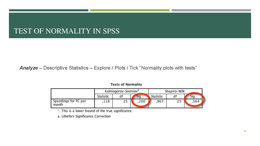
10.

TEST OF NORMALITY IN SPSS
Analyze – Descriptive Statistics – Explore / Plots / Tick “Normality plots with tests”
10

11.

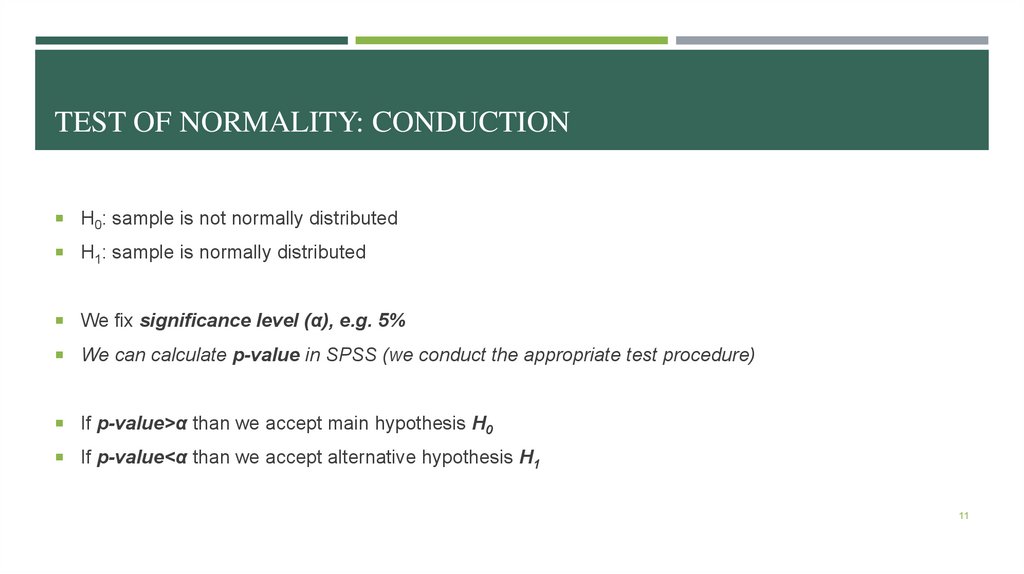
TEST OF NORMALITY: CONDUCTION
H0: sample is not normally distributed
H1: sample is normally distributed
We fix significance level (α), e.g. 5%
We can calculate p-value in SPSS (we conduct the appropriate test procedure)
If p-value>α than we accept main hypothesis H0
If p-value<α than we accept alternative hypothesis H1
11

12.

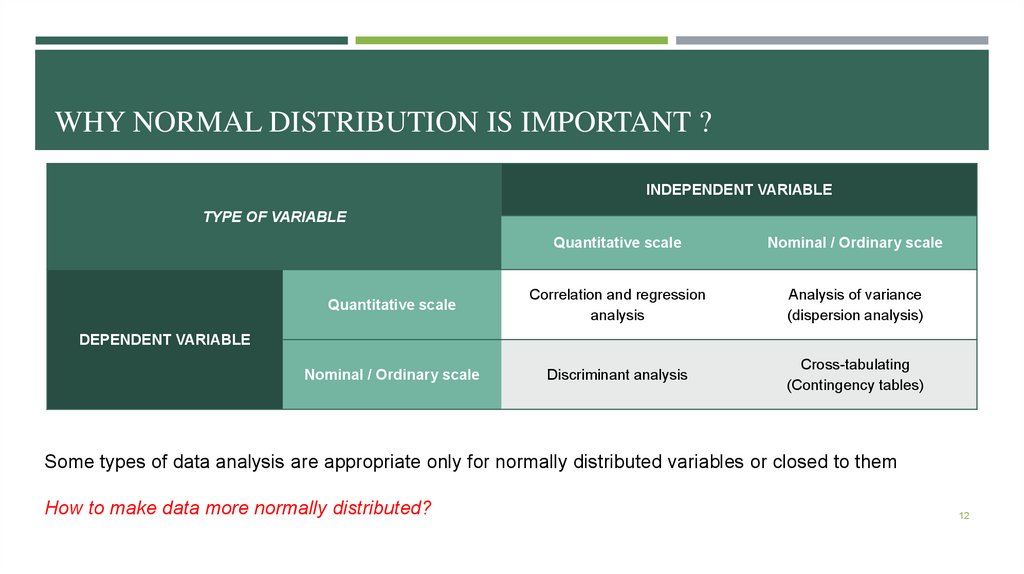
WHY NORMAL DISTRIBUTION IS IMPORTANT ?
INDEPENDENT VARIABLE
TYPE OF VARIABLE
Quantitative scale
Nominal / Ordinary scale
Quantitative scale
Correlation and regression
analysis
Analysis of variance
(dispersion analysis)
Nominal / Ordinary scale
Discriminant analysis
Cross-tabulating
(Contingency tables)
DEPENDENT VARIABLE
Some types of data analysis are appropriate only for normally distributed variables or closed to them
How to make data more normally distributed?
12

13.

DESCRIBING DATA: «FIRST SIGHT ON THE DATA»
Graphical description
E.g., histograms (to identify outlines – «выбросы»)
Numerical descriptive measures
Median, mode
Range, Minimum, Maximum
Mean, Standard deviation
…
13

14.

DESCRIPTIVE STATISTICS
Analysis of the basic statistical parameters in order to get acquainted with the data, to reveal its features, to
correct the hypotheses.
Descriptive statistics is carried out in different ways depending on which scale the variables are
measured in:
-
Nominal
-
Ordinal
-
Quantitative
14

15.

DESCRIPTIVE STATISTICS: MAIN INDICATORS
Mode «мода»
Median «медиана»
Range «размах»
Minimum
Maximum
Mean (=average) «среднее»
Standard deviation «стандартное отклонение»
15

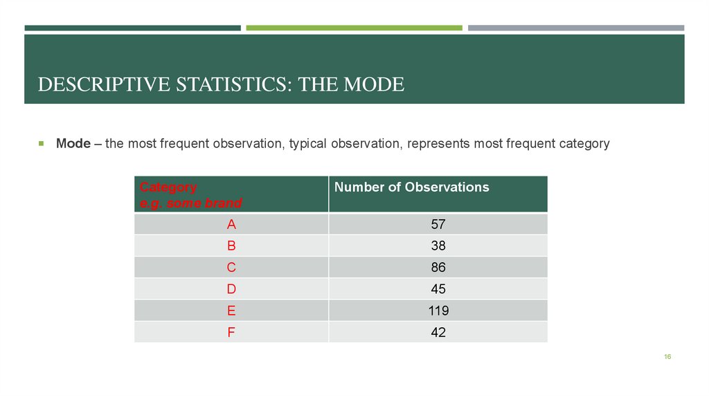
16.

DESCRIPTIVE STATISTICS: THE MODE
Mode – the most frequent observation, typical observation, represents most frequent category
Category
e.g. some brand
Number of Observations
A
57
B
38
C
86
D
45
E
119
F
42
16

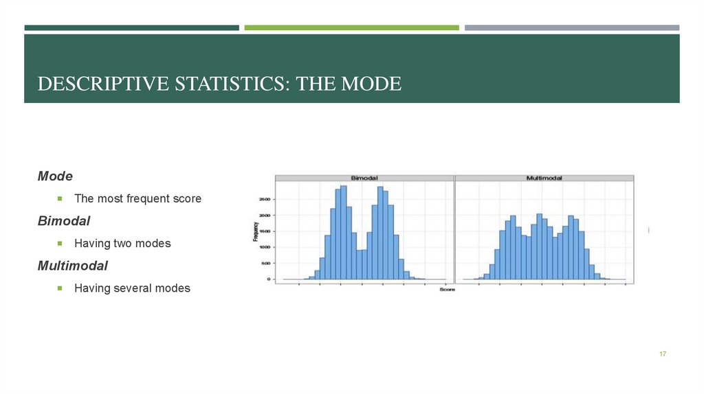
17.

DESCRIPTIVE STATISTICS: THE MODE
Mode
The most frequent score
Bimodal
Having two modes
Multimodal
Having several modes
17

18.

DESCRIPTIVE STATISTICS: THE MEDIAN
Median – the value that is in the middle: half of the observations are higher than
median and half of the observations are lower than median
The median is the middle score when scores are ordered:
Ex. 1. Median(15,27,14,18,21) = Median(14,15,18,21,27) = 18
Ex. 2. Median(15,27,14,18) = Median(14,15,18,27) = (15+18)/2 = 16,5
Category
Number of
Observations
A
57
B
38
C
86
D
45
E
119
F
42
18

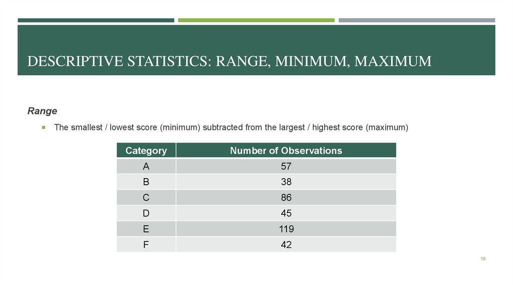
19.

DESCRIPTIVE STATISTICS: RANGE, MINIMUM, MAXIMUM
Range
The smallest / lowest score (minimum) subtracted from the largest / highest score (maximum)
Category
Number of Observations
A
57
B
38
C
86
D
45
E
119
F
42
19

20.

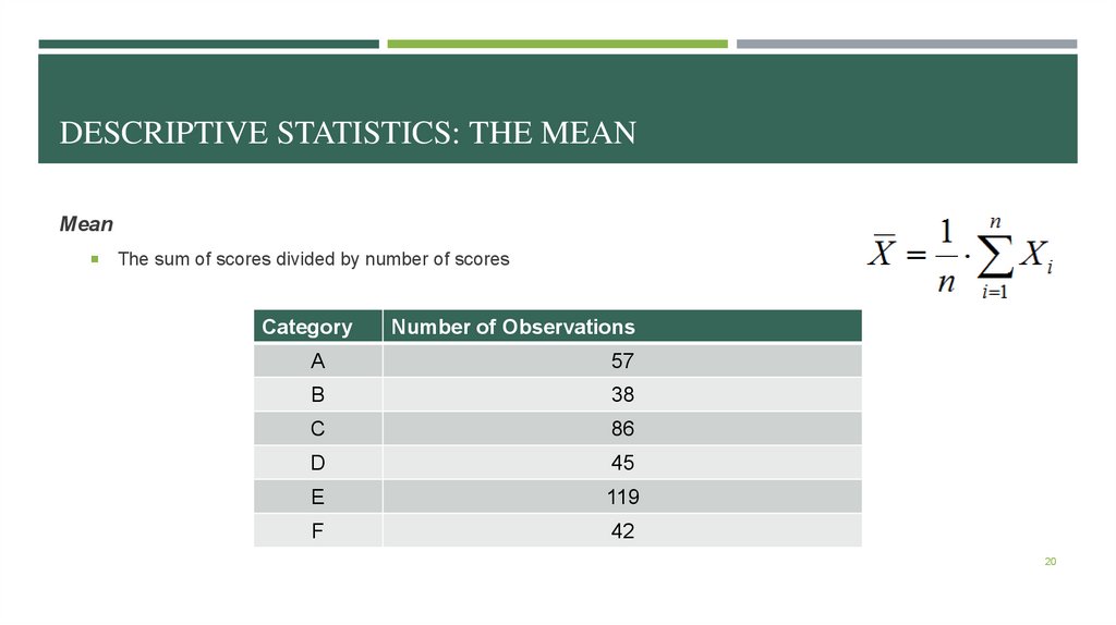
DESCRIPTIVE STATISTICS: THE MEAN
Mean
The sum of scores divided by number of scores
Category
Number of Observations
A
57
B
38
C
86
D
45
E
119
F
42
20

21.

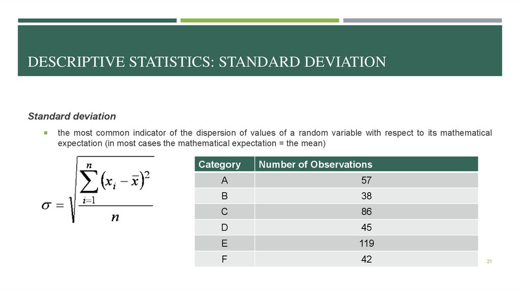
DESCRIPTIVE STATISTICS: STANDARD DEVIATION
Standard deviation
the most common indicator of the dispersion of values of a random variable with respect to its mathematical
expectation (in most cases the mathematical expectation = the mean)
Category
Number of Observations
A
57
B
38
C
86
D
45
E
119
F
42
21

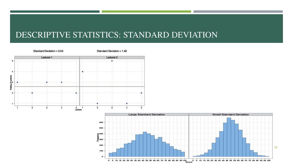
22.

DESCRIPTIVE STATISTICS: STANDARD DEVIATION
22

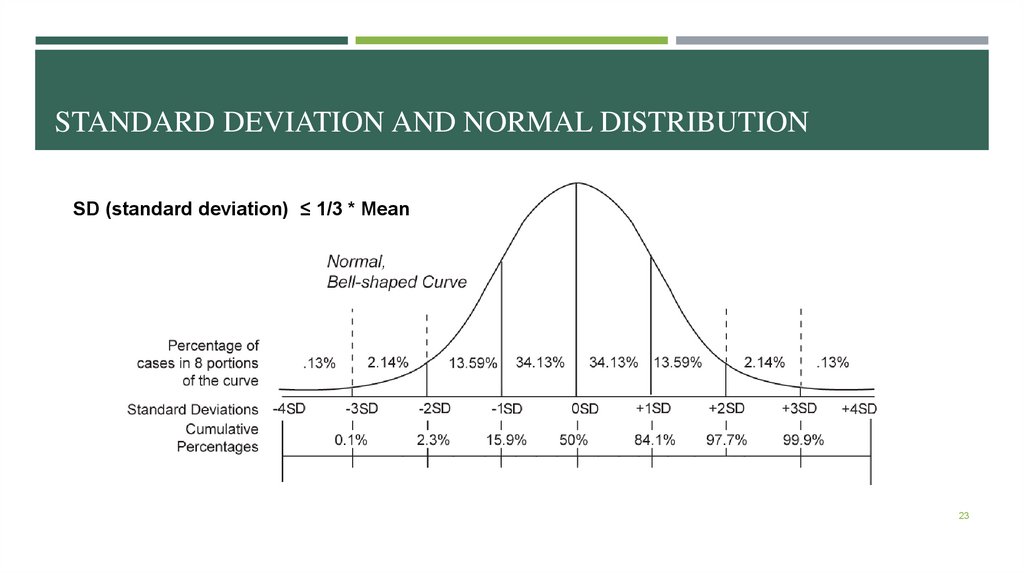
23.

STANDARD DEVIATION AND NORMAL DISTRIBUTION
SD (standard deviation) ≤ 1/3 * Mean
23

24.

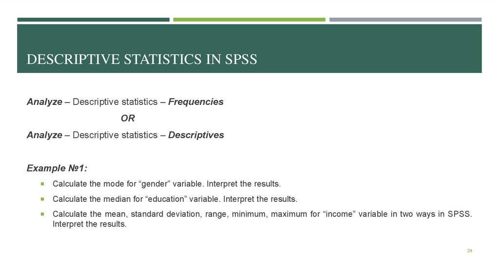
DESCRIPTIVE STATISTICS IN SPSS
Analyze – Descriptive statistics – Frequencies
OR
Analyze – Descriptive statistics – Descriptives
Example №1:
Calculate the mode for “gender” variable. Interpret the results.
Calculate the median for “education” variable. Interpret the results.
Calculate the mean, standard deviation, range, minimum, maximum for “income” variable in two ways in SPSS.
Interpret the results.
24

25.

DESCRIPTIVE STATISTICS FOR VARIABLES IN DIFFERENT SCALES
Nominal – mode
Ordinal – mode + median, mean, standard deviation
Quantitative (Scale) – mode, median, mean, standard deviation + range, minimum, maximum
25

26.

CROSS-TABULATING
(CONTINGENCY TABLES)

27.

CROSS-TABULATING
Contingency tables (or cross tables) are usually constructed in the case when two qualitative (nominal
or ordinal) variables are analyzed and there is a question about the influence of one of them on the
other.
Contingency tables (or cross tables) allow to prove a hypothesis about the relationship between two
qualities (= two qualitative variables).
Contingency tables (or cross tables) is a means of visualizing the joint distribution of two variables. The
general format of a contingency table is a group statistical table. In its rows, the values of one variable
are located, and the values of another variable are displayed in columns.

28.

THE EXAMPLE OF USING CROSS-TABULATING FOR SEGMENTING
THE MARKET
Cust Number of
omer visits a week
Age
Income,
rub.
Educatio
n
1
2
39
> 60 000
bachelor
2
1
63
bachelor
3
4
24
4
7
21
20 000-39
000
20 000-39
000
< 20 000
5
6
26
40 000-60
000
Number
of visits
a week
20
and
less
10%
Age
Sum
21-29 30-39 40-49 50 and
more
master
1 and
less
2-3
5%
15%
30%
40%
100%
5%
20%
35%
25%
15%
100%
master
4-5
15%
35%
25%
20%
5%
100%
bachelor
6 and
more
10%
40%
30%
15%
5%
100%
…
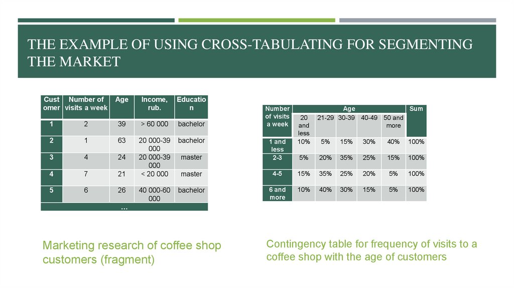
Marketing research of coffee shop
customers (fragment)
Contingency table for frequency of visits to a
coffee shop with the age of customers

29.

THE EXAMPLE OF USING CROSS-TABULATING FOR SEGMENTING
THE MARKET
Cust Number of
omer visits a week
Age
Income,
rub.
Educatio
n
1
2
39
> 60 000
bachelor
2
1
63
bachelor
3
4
24
4
7
21
20 000-39
000
20 000-39
000
< 20 000
5
6
26
40 000-60
000
Number
of visits
a week
20
and
less
10%
Age
Sum
21-29 30-39 40-49 50 and
more
master
1 and
less
2-3
5%
15%
30%
40%
100%
5%
20%
35%
25%
15%
100%
master
4-5
15%
35%
25%
20%
5%
100%
bachelor
6 and
more
10%
40%
30%
15%
5%
100%
…
Marketing research of coffee shop
customers (fragment)
Contingency table for frequency of visits to a
coffee shop with the age of customers

30.

CONTINGENCY TABLES: VISUALIZATION
Put the independent variable on columns and the dependent variable on rows
Percentages are usually more informative, but always report the row/column sums so
that the counts can be reconstructed

31.

CHI-SQUARE TEST
Pearson Chi-Square test is a nonparametric method that allows to check the presence or absence of a
relationship between two qualitative variables
H0: there is no connection between variables
H1: there is connection between variables
If Sig.>0.05 than we accept main hypothesis H0
If Sig.<0.05 than we accept alternative hypothesis H1

32.

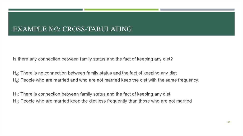
EXAMPLE №2: CROSS-TABULATING
Is there any connection between family status and the fact of keeping any diet?
H0: There is no connection between family status and the fact of keeping any diet
H0: People who are married and who are not married keep the diet with the same frequency.
H1: There is connection between family status and the fact of keeping any diet
H1: People who are married keep the diet less frequently than those who are not married
32

33.

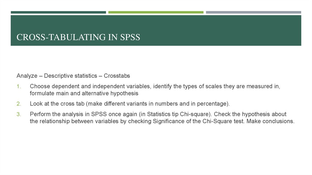
CROSS-TABULATING IN SPSS
Analyze – Descriptive statistics – Crosstabs
1.
Choose dependent and independent variables, identify the types of scales they are measured in,
formulate main and alternative hypothesis
2.
Look at the cross tab (make different variants in numbers and in percentage).
3.
Perform the analysis in SPSS once again (in Statistics tip Chi-square). Check the hypothesis about
the relationship between variables by checking Significance of the Chi-Square test. Make conclusions.

34.

WHAT TO DO WITH THE QUANTITATIVE DATA?..
34

35.

TASK №2
Example №1 or 1-1:
Build possible graphs for this dataset (choosing the most appropriate chart for each variable) + two charts of
comparisons between them
Estimate the descriptive statistics for this dataset (choosing the most appropriate indicators of descriptive
statistics for each variable)
Formulate 3 hypotheses that can be tested using the cross-tabulating method. Verify hypotheses by making
necessary calculations (* use a quantitative variable in at least 1 hypothesis)
Make some conclusions about the data
All results should be presented on one .doc file
35