System analysis and decision making Decision Trees

1.

System analysis and decision making
Decision Trees

2.

System analysis and decision making
The systematic use of trees for knowledge
representation can be used for fast and
frugal decisions.
Tree-structured schemes are ubiquitous
tools for organising and representing
knowledge.

3.

System analysis and decision making
Bayesian model

4.

System analysis and decision making
Probabilistic Modelling
-A model describes data that one
could observe from a system,
-If we use the mathematics of
probability theory to express all
forms of uncertainty and noise
associated with our model...
- ...then inverse probability (i.e.
Bayes rule) allows us to infer
unknown quantities, adapt our

5.

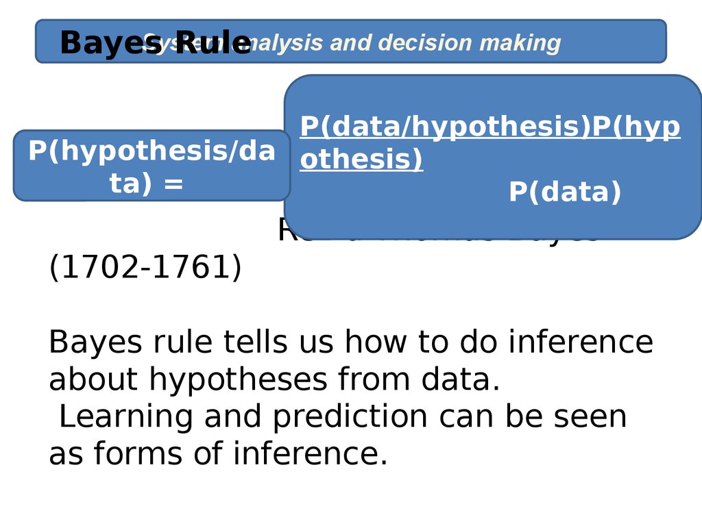
System
analysis and decision making
Bayes
Rule
P(data/hypothesis)P(hyp
P(hypothesis/da othesis)
ta) =
P(data)
Rev'd Thomas Bayes
(1702-1761)
Bayes rule tells us how to do inference
about hypotheses from data.
Learning and prediction can be seen
as forms of inference.

6.

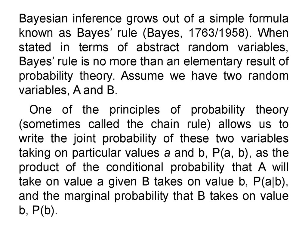
Bayesian inference grows out of a simple formula
known as Bayes’ rule (Bayes, 1763/1958). When
stated in terms of abstract random variables,
Bayes’ rule is no more than an elementary result of
probability theory. Assume we have two random
variables, A and B.
One of the principles of probability theory
(sometimes called the chain rule) allows us to
write the joint probability of these two variables
taking on particular values a and b, P(a, b), as the
product of the conditional probability that A will
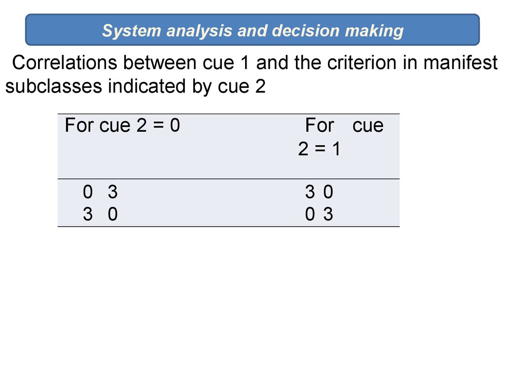
take on value a given B takes on value b, P(a|b),
and the marginal probability that B takes on value
b, P(b).

7.

System analysis and decision making
Thus, we have
P(a, b) = P(a|b)P(b). (1)
There was nothing special about the choice of A
rather than B in factorizing the joint probability in
this way, so we can also write P(a, b) = P(b|a)P(a).
(2)
It follows from Equations 1 and 2 that P(a|b)P(b) =
P(b|a)P(a), which can be rearranged to give P(b|a)
= P(a|b)P(b)
P(a)
. (3)
This expression is Bayes’ rule, which indicates how
we can compute the conditional probability of b
given a from the conditional probability of a given b.

8.

System analysis and decision making
The both full Bayesian inference and onereason decision making are processes that
can be described in terms of treestructured decision rules.
A fully specified Bayesian model can be
represented by means of the “full” or
“maximal” tree obtained by introducing
nodes for all conceivable conjunctions of
events, whereas one-reason decision rule
can be represented by a “minimal” subtree
of the maximal tree (with maximal and

9.

Subtrees of the full tree not containing any path
from a root to leaves are regarded as “truncated”
since they necessarily truncate the access to
available information.
Minimal trees can be obtained by radically
pruning the full tree. A minimal tree has a leaf at
each one of its levels, so that every level allows
for a possible decision.

10.

System analysis and decision making
Indeed, when a radical reduction of complexity is
necessary and when the environment is
favorable, such a minimal tree will be extremely
fast and frugal with negligible losses in accuracy.
А name for such minimal trees is “fast and
frugal trees”.

11.

System analysis and decision making
TREE-STRUCTURED
REPRESENTATIONS IN
CLASSIFICATION TASKS

12.

System analysis and decision making
Human classifications and decisions are based on
the analysis of features or cues that the mind/brain
extracts from the environment.
There is a wide spectrum of classification schemes,
varying in terms of the time scale they require, from
almost automatic classifications the mind/brain
performs without taking real notice, up to slow,
conscious ones.

13.

System analysis and decision making
Among the diverse representation a device for
classification, trees have been the most ubiquitous.
Since the fourth century, trees representing
sequential step-by-step processes for classification
based on cue information have been common
devices in many realms of human knowledge.
These trees start from a root node and descend
through branches connecting the root to intermediate
nodes until they reach final nodes or leaves.

14.

System analysis and decision making
A classification (also called categorization) tree is a
graphical representation of a rule - or a set of rules
- for making classifications.
Each node of the tree represents a question
regarding certain features of the objects to be
classified or categorized.
Each branch leading out of the node represents a
different answer to the question.
It is assumed that the answers to the question
are exclusive (non-overlapping) and exhaustive
(cover all objects).

15.

System analysis and decision making
That is, there is exactly one answer to the question
for each object, and each of the possible answers
is represented by one branch out of the node.
The nodes below a given node are called its
“children”, and the node above a node is called its
“parent”.
Every node has exactly one parent except for the
“root” node, which has no parent, and which is
usually depicted at the top or far left. The “leaf”
nodes, or nodes having no children, are usually
depicted at the bottom or far right.

16. In a “binary” tree, all non-leaf nodes have exactly two children; in general trees nodes may have any number of children. The

System analysis and decision making
In a “binary” tree, all non-leaf nodes have
exactly two children; in general trees nodes
may have any number of children.
The leaf nodes of a classification tree represent
a “partition” of the set of objects into classes
defined by the answers to the questions.
Each leaf node has an associated class label,
to be assigned to all objects for which the
appropriate answers are given to the questions
associated with the leaf’s ancestor nodes.

17.

System analysis and decision making
The classification tree can be used to
construct a simple algorithm for associating
any object with a class label.
Given an object, the algorithm traversesa
“path” from the root node to one of the leaf
nodes. This path is determined by the
answers to the questions associated with
the nodes.
The questions and answers can be used to
define a “decision rule” to be executed
when each node is traversed. The decision
rule instructs the algorithm which arc to
traverse out of the node, and thus which

18. Algorithm TREE-CLASS: Begin at root node. Execute rule associated with current node to decide which arc to traverse. Proceed to

System analysis and decision making
Algorithm TREE-CLASS:
Begin at root node.
Execute rule associated with current node to decide
which arc to traverse.
Proceed to child at end of chosen arc.
If child is a leaf node, assign to object the class label
associated with node and STOP.
Otherwise, go to (2).

19.

System analysis and decision making
Natural Frequency
Trees
Natural frequency trees provide good
representations of the statistical data relevant
to the construction of optimal classification
trees.

20.

System analysis and decision making

21.

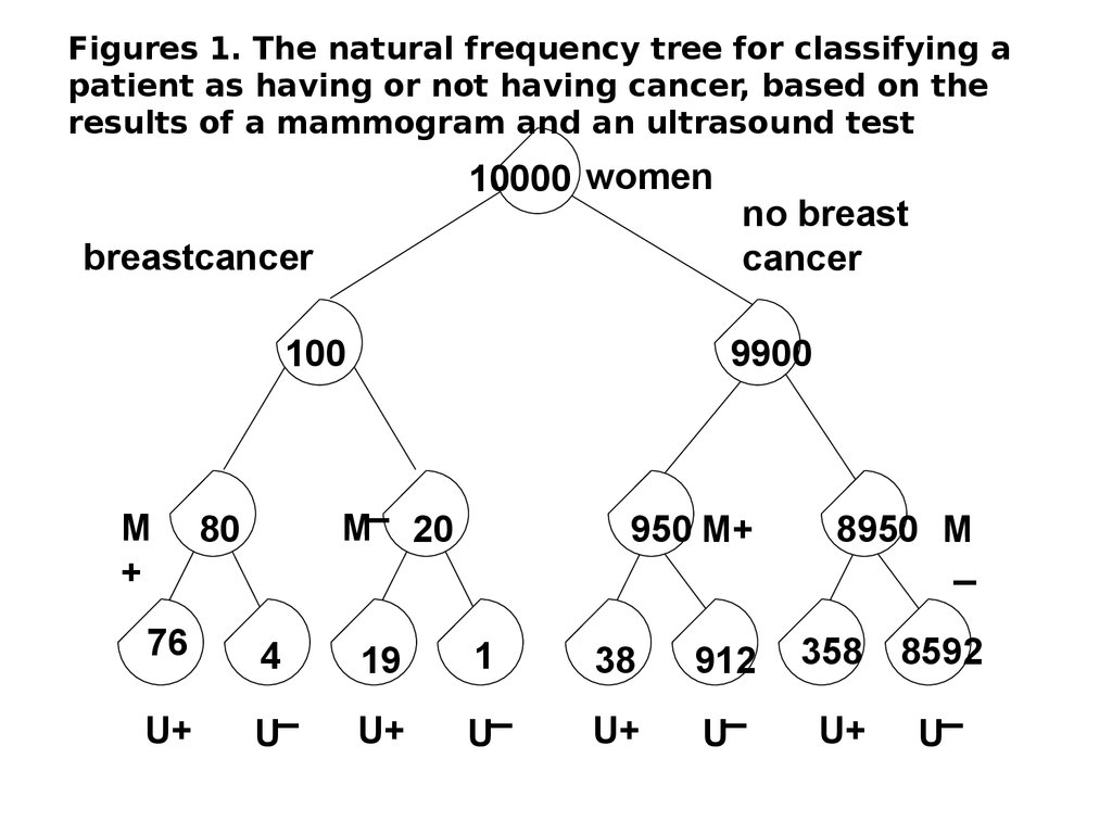
Figures 1. The natural frequency tree for classifying a
patient as having or not having cancer, based on the
results of a mammogram and an ultrasound test
10000 women
breastcancer
100
M
+
9900
M− 20
80
no breast
cancer
950 M+
8950 M
−
76
4
19
1
38
912
358
U+
U−
U+
U−
U+
U−
U+
8592
U−

22.

How many of the women who get a positive
mammography and a positive ultrasound test do
you expect to actually have breast cancer?

23.

System analysis and decision making
“Natural frequency tree”.
The numbers in the nodes indicate that the two
tests are conditionally independent, given cancer.
This is obviously an assumption the reality of
medical tests is that neither combined
sensitivities nor combined specificities are
reported in the literature.
It is a frequent convention to assume tests’
conditional independence, given the disease.

24.

System analysis and decision making
There are more practical natural frequency trees
for diagnosis.
They are obtained by inverting the order followed
for the sequential partitioning of the total
population (10000 women)

25.

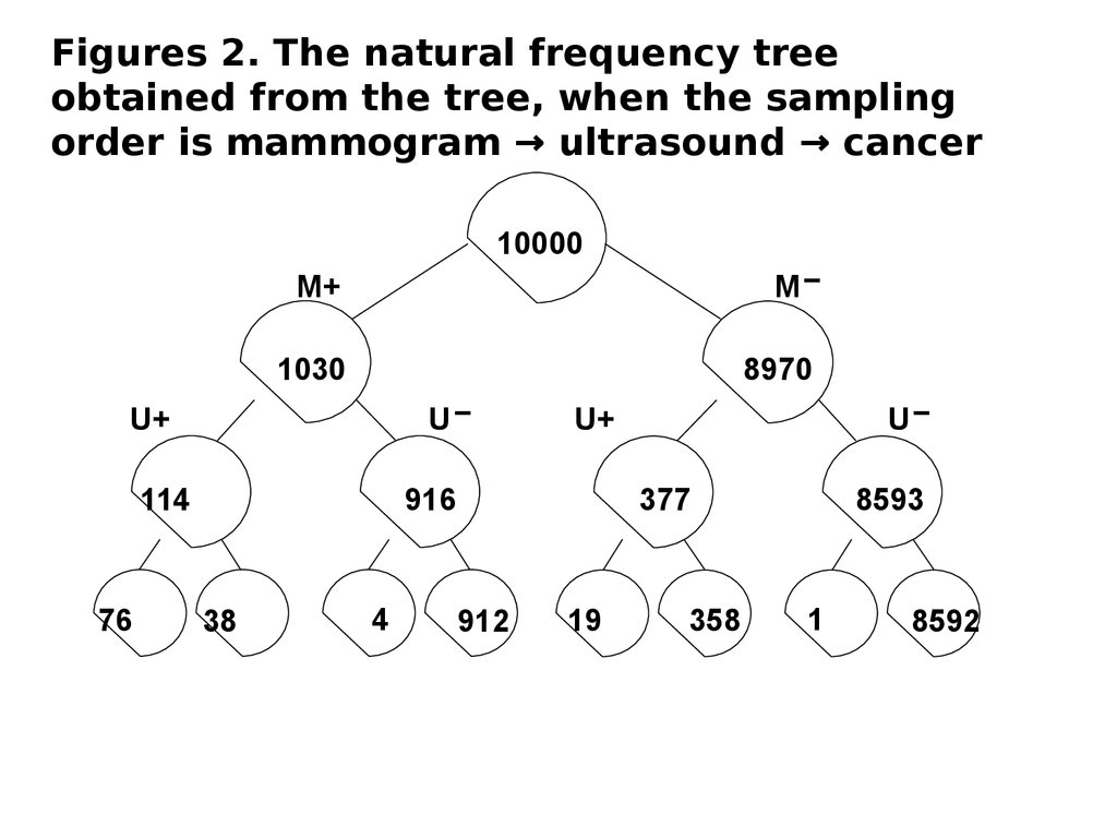
Figures 2. The natural frequency tree
obtained from the tree, when the sampling
order is mammogram → ultrasound → cancer
10000
M+
M−
1030
8970
U−
U+
114
76
916
38
4
U−
U+
377
912
19
358
8593
1
8592

26. Organizing the tree in the diagnostic direction produces a much more efficient classification strategy. This tree has two major

advantages over the
tree in Figure 1. for a diagnostic task.
First, we can follow the TREE-CLASS algorithm
for the first two steps before becoming stuck at
the second-to-last level above the leaf nodes.
For example, for the hypothetical woman with
M+ and U+ described above, we would be able
to place her among the 114 women at the
leftmost node on the third level from the top.

27.

System analysis and decision making
Second, once we have placed a patient at a
node just above the bottom of the tree, we can
compute the probability of placing her at each
of the two possible leaf nodes by using only
local information.

28. That is, the probability comparing the leaves of Figures 1 and 2 reveals that they are the same. That is, they contain the same

System analysis and decision making
That is, the probability comparing
the leaves of Figures 1 and 2 reveals
that they are the same.
That is, they contain the same
numbers, although their ordering is
different, as is the topology of their
connection to the rest of the tree.
One might question whether a
natural sampler would partition the
population in the causal or the
diagnostic direction.

29.

System analysis and decision making
Knowledge tends to be organised
causally, and diagnostic inference is
performed by means of inversion
strategies, which, in the frequency
format, are reduced to inventing the
partitioning order as above
(in the probability format, the
inversion is carried out by applying
Bayes’ theorem).

30.

System analysis and decision making
However, ecologically situated agents
tend to adopt representations tailored
to their goals and the environment in
which they are situated.
Thus, it might be argued that a goaloriented natural sampler performing a
diagnostic task will probably partition
the original population according to
the cues first, and end by partitioning
according to the criterion.

31.

System analysis and decision making
Now, consider another version of the
diagnostic ordering of the cues, where, in
the first phase, women are partitioned
according to their ultrasound, and in the
second phase, they are partitioned
according to the mammograms and
finally according to breast cancer.
The tree is depicted in Figure 3.

32.

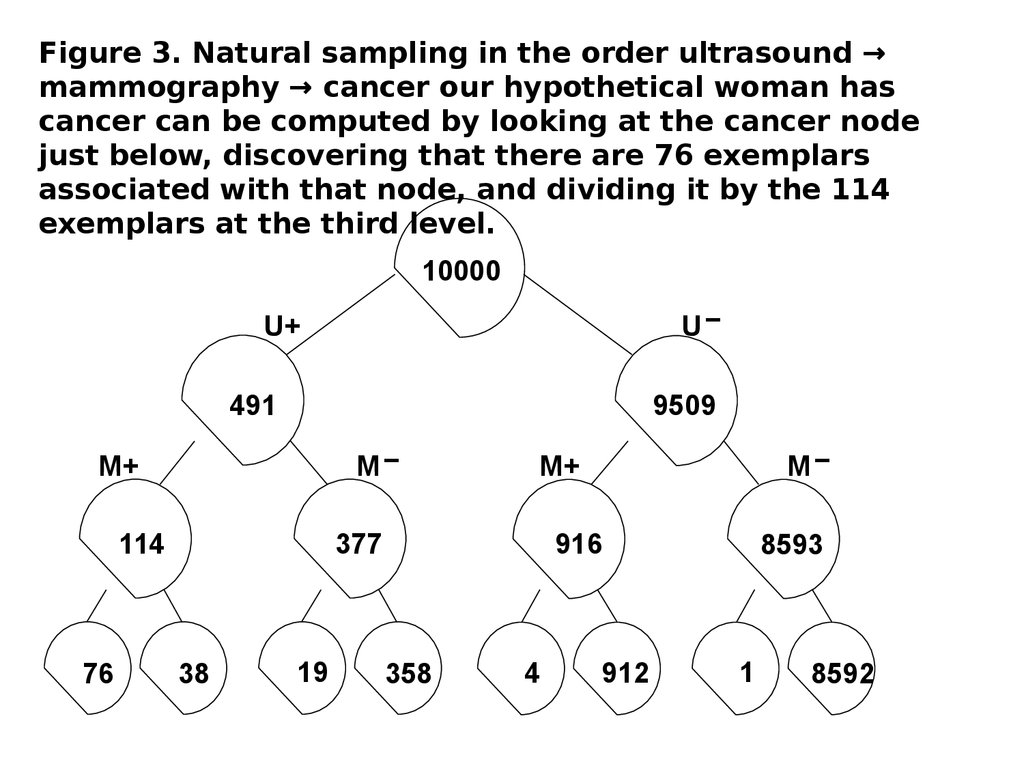
Figure 3. Natural sampling in the order ultrasound →
mammography → cancer our hypothetical woman has
cancer can be computed by looking at the cancer node
just below, discovering that there are 76 exemplars
associated with that node, and dividing it by the 114
exemplars at the third level.
10000
U−
U+
491
9509
M−
M+
114
76
377
38
19
M−
M+
916
358
4
912
8593
1
8592

33.

System analysis and decision making
FAST AND FRUGAL TREES
A tree may be called a fast and frugal tree, that is,
trees constructed with binary cues and a binary
criterion.
The
generalisation
to
other
cases
is
straightforward. With the classification according
to a binary criterion (for example, “cancer” or “no
cancer”), we associate two possible decisions,
one for each possible classification (for example,
“biopsy” or “no biopsy”).

34.

System analysis and decision making
An important convention has to be applied
beforehand: cue profiles can be expressed
as vectors of 0s and 1s, where a 1
corresponds to the value of the cue more
highly correlated with the outcome of the
criterion
considered
“positive”
(for
example, a presence of cancer).
The convention is that left branches are
labelled with 1s and right branches with 0s.
Thus, each branch of the fully specified tree
can be labelled with a 1 or a 0, according to

35.

System analysis and decision making
Definition
A fast and frugal binary decision tree is
a decision tree with at least one exit
leaf at every level. That is, for every
checked cue, at least one of its
outcomes can lead to a decision.
In accordance with the convention
applied above, if a leaf stems from a
branch labelled 1, the decision will be

36.

System analysis and decision making
We begin by recalling that according to our
convention, we will encode “having the disease”
with a 1, and “not having the disease” with a 0.
If we have, say, three cues, the leaves of the full
frequency tree will be labeled (111,1), (111,0),
(101,1), (101,0), (100,1), (100,0), (011,1),
(011,0), (010,1), (010,1), (001,0), (000,1),
(000,0), where the binary vectors will appear in
decreasing lexicographic order from left to right.
Observe that the cue profile from the state of the
disease is separated by a comma.

37.

System analysis and decision making
Since this ordering is similar to the ordering
of words in a dictionary, it is usually called
“lexicographic”.
Lexicographic orderings allow for simple
classifications, by establishing that all
profiles larger (in the lexicographic ordering)
than a certain fixed profile will be assigned to
one class, and all profiles smaller than the
same fixed profile will be assigned to the
other class.

38.

A lexicographic classifier determined by the path of
profile (101), where the three bits are cue values and
the last bit corresponds to the criterion (for example,
having or not having the disease)
(111,1)
(111,0) 110,1)
(110,0) (101,1) (101,0) (100,1)
(100,0)
(011,1)
(011,0) (010,1) (010,0) (001,1) (001,0)( 000,1) (000,0)

39.

System analysis and decision making
A “lexicographic decision rule” makes one
decision, say, D, for all profiles larger than a
given, fixed profile, and the alternative
decision, ¬D, for all profiles smaller than that
same profile.
The profile itself is assigned decision D if it
ends with a 1, and decision ¬D if it ends with
a 0.
A fast and frugal decision tree makes
decisions lexicographically. This is what we

40.

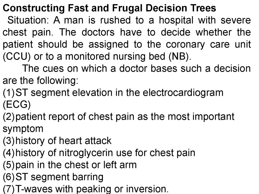
Constructing Fast and Frugal Decision Trees
Situation: A man is rushed to a hospital with severe
chest pain. The doctors have to decide whether the
patient should be assigned to the coronary care unit
(CCU) or to a monitored nursing bed (NB).
The cues on which a doctor bases such a decision
are the following:
(1)ST segment elevation in the electrocardiogram
(ECG)
(2)patient report of chest pain as the most important
symptom
(3)history of heart attack
(4)history of nitroglycerin use for chest pain
(5)pain in the chest or left arm
(6)ST segment barring
(7)T-waves with peaking or inversion.

41.

Green and Mehr (1997) analyzed the problem of finding
a simple procedure for determining an action based on
this cue information. They reduced the seven cues to
only three (creating a new cue formed by the
disjunction of 3, 4, 6 and 7) and proposed the tree
depicted ST
in segment
Figure.elevation
yes
CCU
no
Chest pain as chief symptom
no
yes
3 or 4 or 6 or 7 is positive
yes
no
CCU
NB
NB

42.

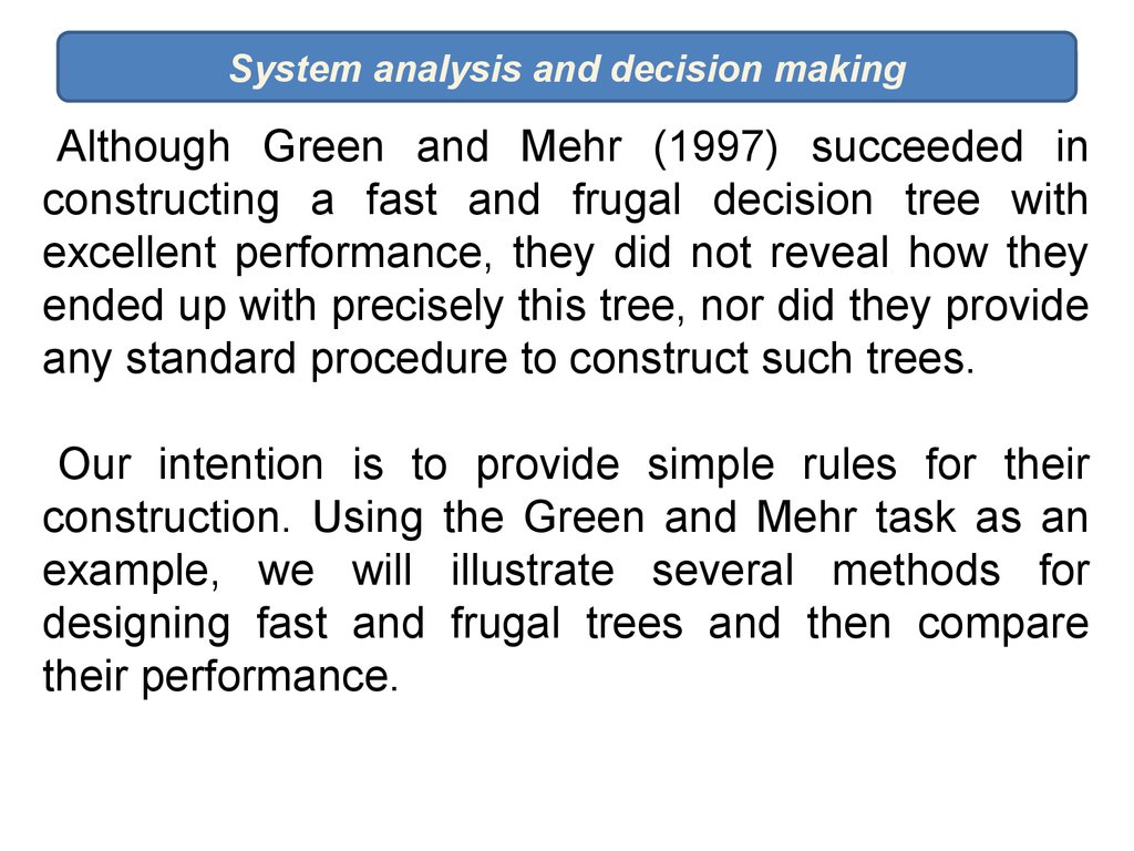
System analysis and decision making
Although Green and Mehr (1997) succeeded in
constructing a fast and frugal decision tree with
excellent performance, they did not reveal how they
ended up with precisely this tree, nor did they provide
any standard procedure to construct such trees.
Our intention is to provide simple rules for their
construction. Using the Green and Mehr task as an
example, we will illustrate several methods for
designing fast and frugal trees and then compare
their performance.

43.

System analysis and decision making
In order to construct a fast and frugal tree,
one can, of course, test all possible
orderings of cues and shapes of trees on
the provided data set and optimize fitting
performance; in the general case, this
requires enormous computation if the
number of cues is large.
Another approach is to determine the
“best” cue according to some given rule,
and then determine the “second best” cue
conditional on the first, and so on. But this

44.

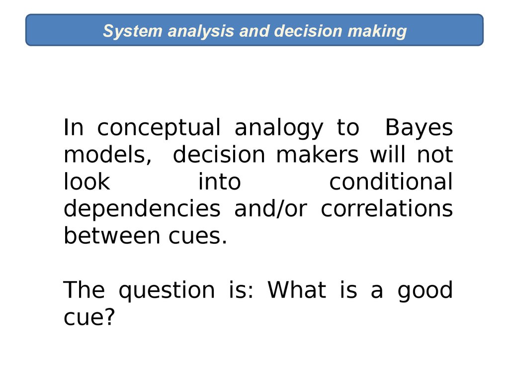
System analysis and decision making
In conceptual analogy to Bayes
models, decision makers will not
look
into
conditional
dependencies and/or correlations
between cues.
The question is: What is a good
cue?

45.

System analysis and decision making
The Shape of Trees
There are four possible shapes, or branching
structures, of fast and frugal trees for three cues.

46.

System analysis and decision making

47.

System analysis and decision making
Trees of type 1 and 4 are called
“rakes” or “pectinates”.
As defined here, rakes have a very
special property.
They embody a strict conjunction rule,
meaning that one of the two alternative
decisions is made only if all cues are
present (type 1) or absent (type 4).

48.

System analysis and decision making
Trees of types 2 and 3 are called
“zigzag trees”.
They
have
the
property
of
alternating between positive and
negative exits in the sequence of
levels.

49. Cue interactions go beyond the bivariate contingencies that are typically observed in the naive (unconditional) linear model

System analysis and decision making
Cue interactions go beyond the bivariate
contingencies that are typically observed in
the naive (unconditional) linear model
framework.
A straightforward demonstration of the
interaction effect is given by what is now
called “Meehl’s paradox” (after its initial
description by the clinician-statistician Paul E.
Meehl, one of the pioneers in the field of
clinical decision making, 1950).

50.

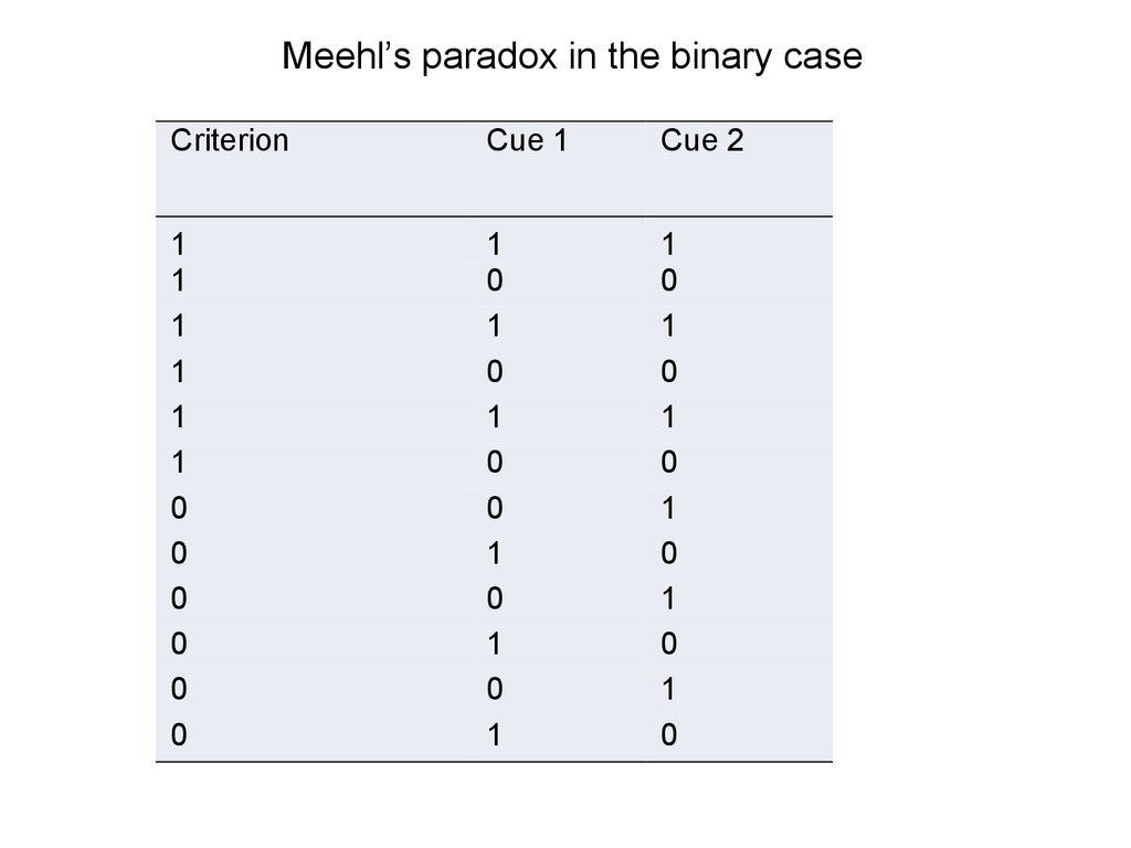
Meehl’s paradox in the binary case
Criterion
Cue 1
Cue 2
1
1
1
1
1
1
0
0
0
0
0
0
1
0
1
0
1
0
0
1
0
1
0
1
1
0
1
0
1
0
1
0
1
0
1
0

51.

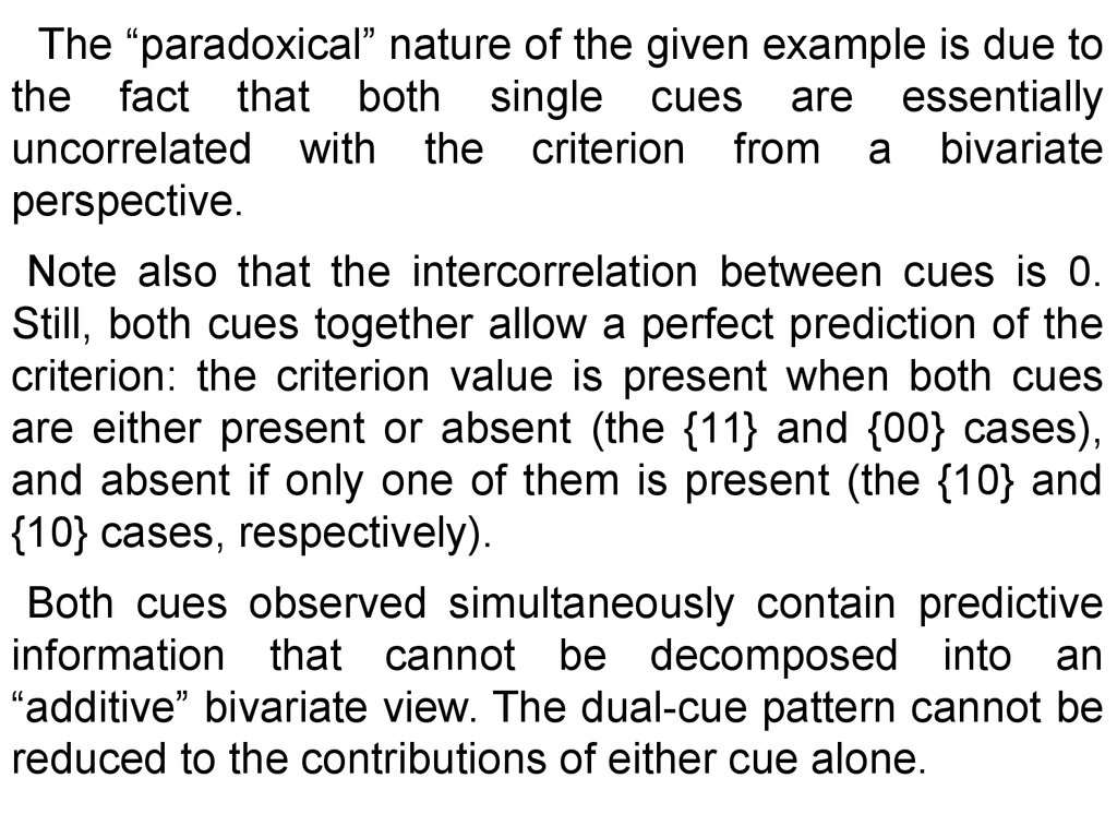
The “paradoxical” nature of the given example is due to
the fact that both single cues are essentially
uncorrelated with the criterion from a bivariate
perspective.
Note also that the intercorrelation between cues is 0.
Still, both cues together allow a perfect prediction of the
criterion: the criterion value is present when both cues
are either present or absent (the {11} and {00} cases),
and absent if only one of them is present (the {10} and
{10} cases, respectively).
Both cues observed simultaneously contain predictive
information that cannot be decomposed into an
“additive” bivariate view. The dual-cue pattern cannot be
reduced to the contributions of either cue alone.

52.

System analysis and decision making
Correlations between cue 1 and the criterion in manifest
subclasses indicated by cue 2
For cue 2 = 0
0 3
3 0
For cue
2=1
30
03

53.

System analysis and decision making
Another way to put it is to look at one of
the two cues as a classifier that
discriminates between those cases where
the correlation between the other cue and
the criterion is positive and those where it
is negative.
The dataset is a mixture of cases with
either positive or negative intercorrelation
between one cue and the criterion, with
the other cue indicating the type of
contingency

54.

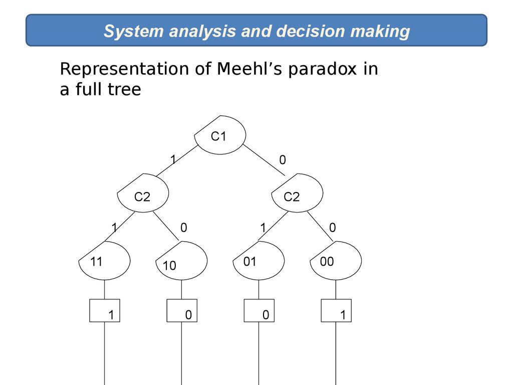
System analysis and decision making
Representation of Meehl’s paradox in
a full tree
C1
1
0
C2
C2
1
11
0
01
10
1
1
0
0
00
0
1

55.

System analysis and decision making
Simple trees bet on a certain structure of the
world, irrespective of the small fluctuations
in a given set of available data.
This can be a major advantage
generalisation if the stable part of
process, which also holds for new data
new environments, is recognised
modelled.
for
the
and
and

56.

System analysis and decision making
From a statistical point of view, it would, of
course, be preferable to testempirically
such assumptions in stead of boldly
implementing them in the model.
But in real-life decision making, we
usually do not have large numbers of data
that are representative of the concrete
decisional setting of interest at our
disposal.

57.

System analysis and decision making
For instance, even for large
epidemiological trials in medicine,
it often remains unclear whether
the resulting databases allow good
generalisation to the situation in a
particular hospital (due to special
properties
of
local
patients,
insufficient
standardisation
of
measurements
and
diagnostic
procedures, etc.).

58.

System analysis and decision making
The fact that cue interactions can exist,
and that they can be covered only by
fully branched tree substructures, does
not imply that they must exist; it says
nothing about the frequency of their
occurrence.
Depending on the kind of the decision
problem, there may be cases where we
can make a reasonable guess about
existing interactions on the substantial
grounds four knowledge of the problem
domain. This may, for instance, be the

59.

System analysis and decision making