Association analysis

1. Association analysis

Naive algorithm
Apriori algorithm
Multilevel association rules discovery
1

2.

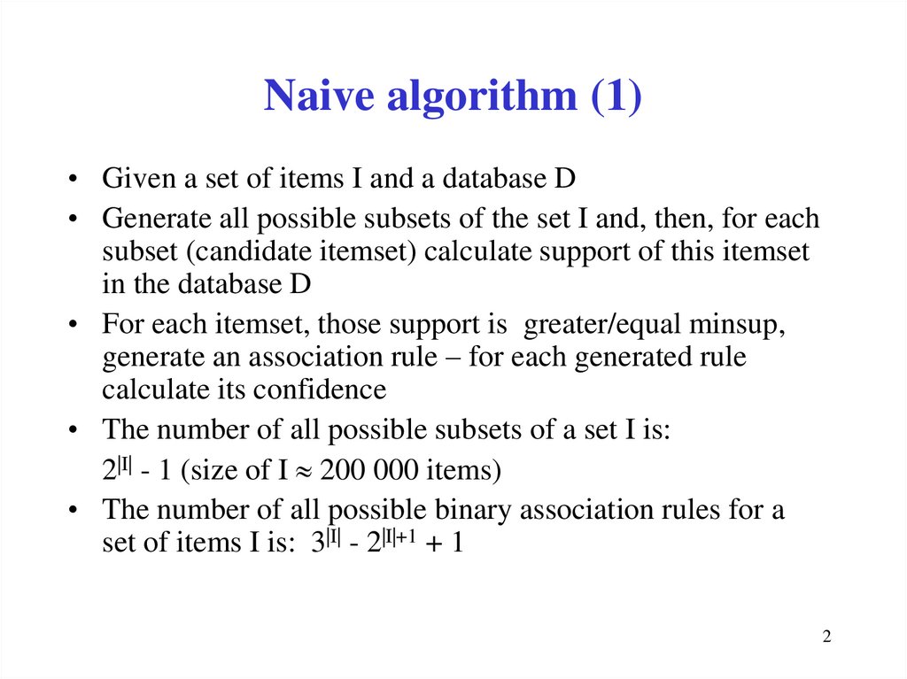
Naive algorithm (1)
• Given a set of items I and a database D
• Generate all possible subsets of the set I and, then, for each
subset (candidate itemset) calculate support of this itemset
in the database D
• For each itemset, those support is greater/equal minsup,
generate an association rule – for each generated rule
calculate its confidence
• The number of all possible subsets of a set I is:
2|I| - 1 (size of I 200 000 items)
• The number of all possible binary association rules for a
set of items I is: 3|I| - 2|I|+1 + 1
2

3.

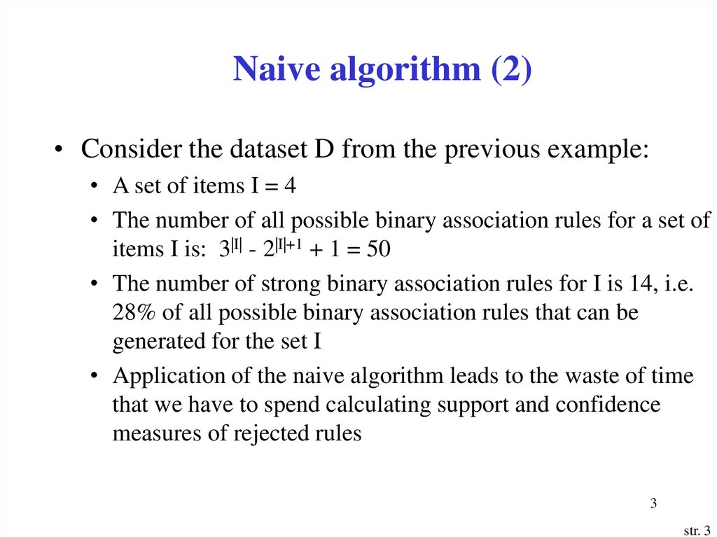
Naive algorithm (2)
• Consider the dataset D from the previous example:
• A set of items I = 4
• The number of all possible binary association rules for a set of
items I is: 3|I| - 2|I|+1 + 1 = 50
• The number of strong binary association rules for I is 14, i.e.
28% of all possible binary association rules that can be
generated for the set I
• Application of the naive algorithm leads to the waste of time
that we have to spend calculating support and confidence
measures of rejected rules
3
str. 3

4.

Naive algorithm (3)
• How can we restrict a number of generated association rules to
avoid the necessity of calculating support and confidence of
rejected rules?
• Answer: it is necessary to consider separately minimum support
and minimum confidence thresholds while generating association
rules
• Notice that the support of a rule X Y is equal to the support
of the set (X, Y)
4
str. 4

5.

Naive algorithm (4)
• If the support of the set (X, Y) is less than minsup, then we may
skip the calculation of the confidence of rules X Y
and Y X
• If the support of the set (X, Y, Z) is less than minsup then we may
skip the calculation of the confidence of rules:
X Y, Z
X, Y Z
Y X, Z
X, Z Y
Z X, Y
Y, Z X
• In general, if the support of a set (X1, X2, …, Xk) is less than
minsup, sup(X1, X2, …, Xk) < minsup, we may skip the
calculation of the confidence of 2k - 2 association rules
5
str. 5

6. General algorithm of association rule discovery

Algorithm 1.1: General algorithm of association
rule discovery
• Find all sets of items Li={Ii1, Ii2, ..., Iim}, Li I, that have
sup(Li) minsup. Sets Li are called frequent itemsets.
• Use the frequent itemsets to generate the association rules
using the algorithm 1.2.
6

7. Rule Generation Algorithm

Algorithm 1.2: Rule generation.
for each frequent itemset Li do
for each subset subLi of Li do
if support(Li)/support(subLi) minconf then
output the rule subLi (Li-subLi)
with confidence = support(Li)/support(subLi)
and support = support(Li)
7

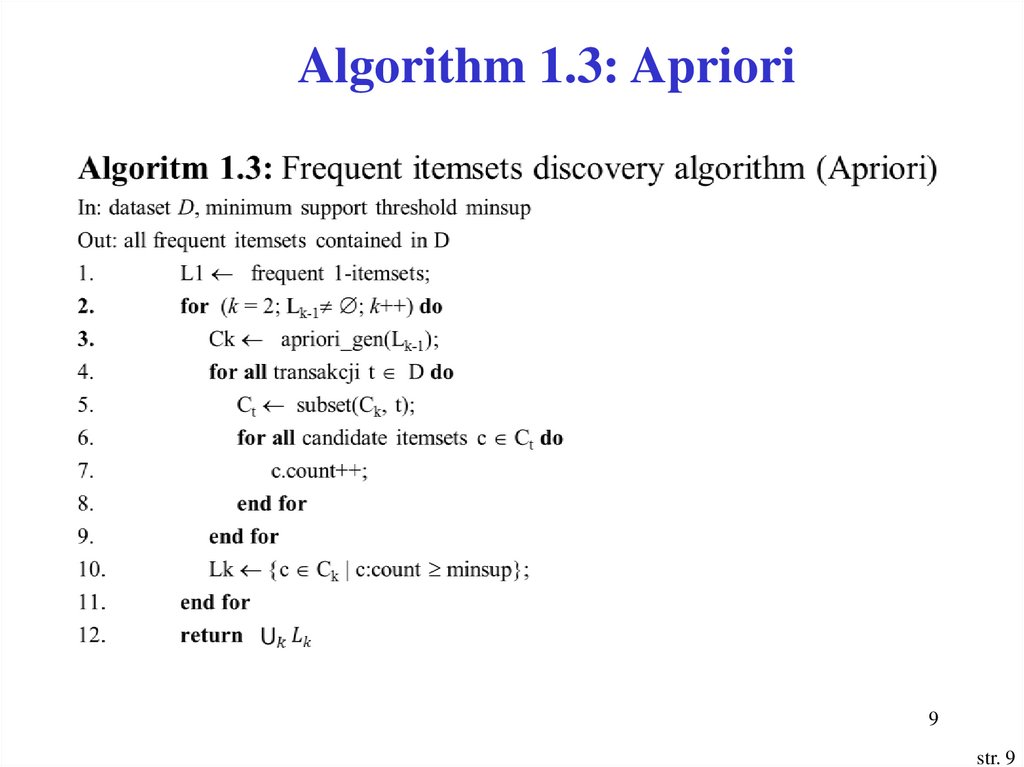
8. Algorithm 1.3: Apriori

Notation:
Assume that all transactions are internally ordered
Lk denotes a set of frequent itemsets of size k (those
with minimum support) – frequent k-itemsets
Ck denotes a set of candidate itemsets of size k
(potentially frequent itemsets) – candidate k- itemsets
8

9.

Algorithm 1.3: Apriori
9
str. 9

10.

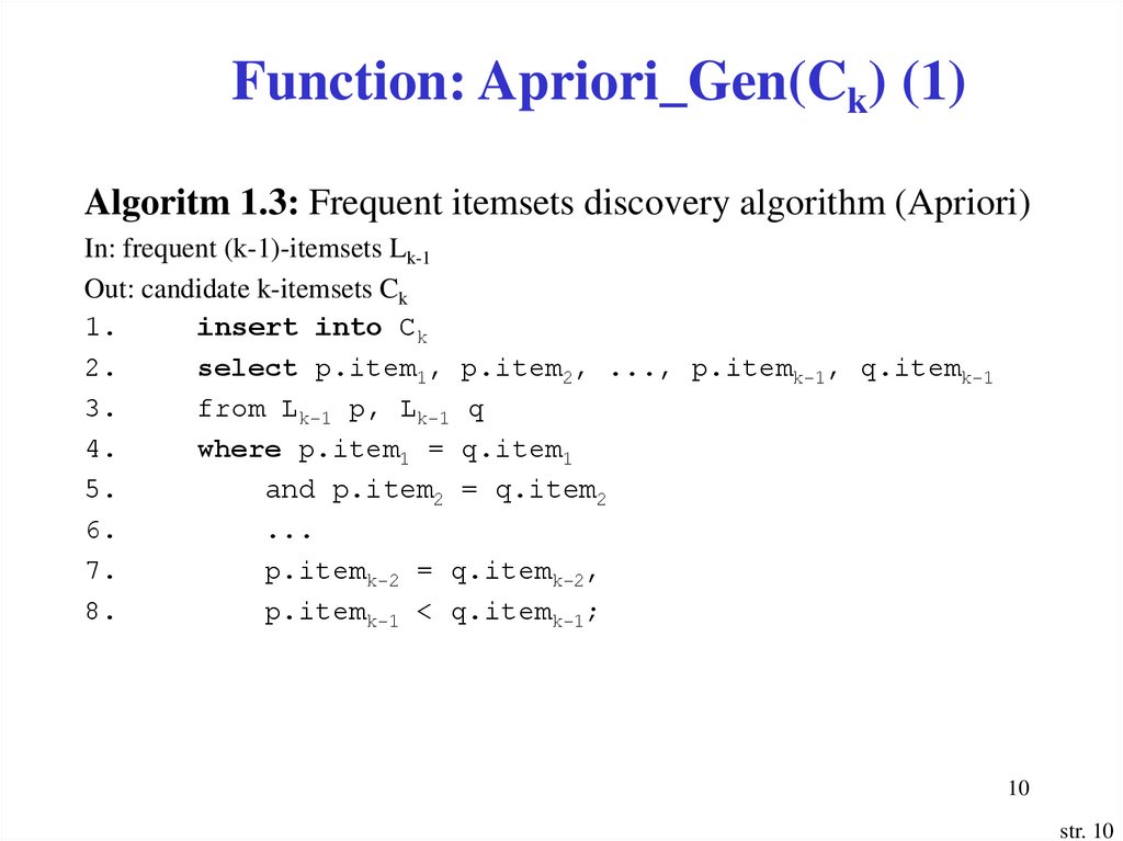
Function: Apriori_Gen(Ck) (1)
Algoritm 1.3: Frequent itemsets discovery algorithm (Apriori)
In: frequent (k-1)-itemsets Lk-1
Out: candidate k-itemsets Ck
1.
insert into Ck
2.
select p.item1, p.item2, ..., p.itemk-1, q.itemk-1
3.
from Lk-1 p, Lk-1 q
4.
where p.item1 = q.item1
5.
and p.item2 = q.item2
6.
...
7.
p.itemk-2 = q.itemk-2,
8.
p.itemk-1 < q.itemk-1;
10
str. 10

11.

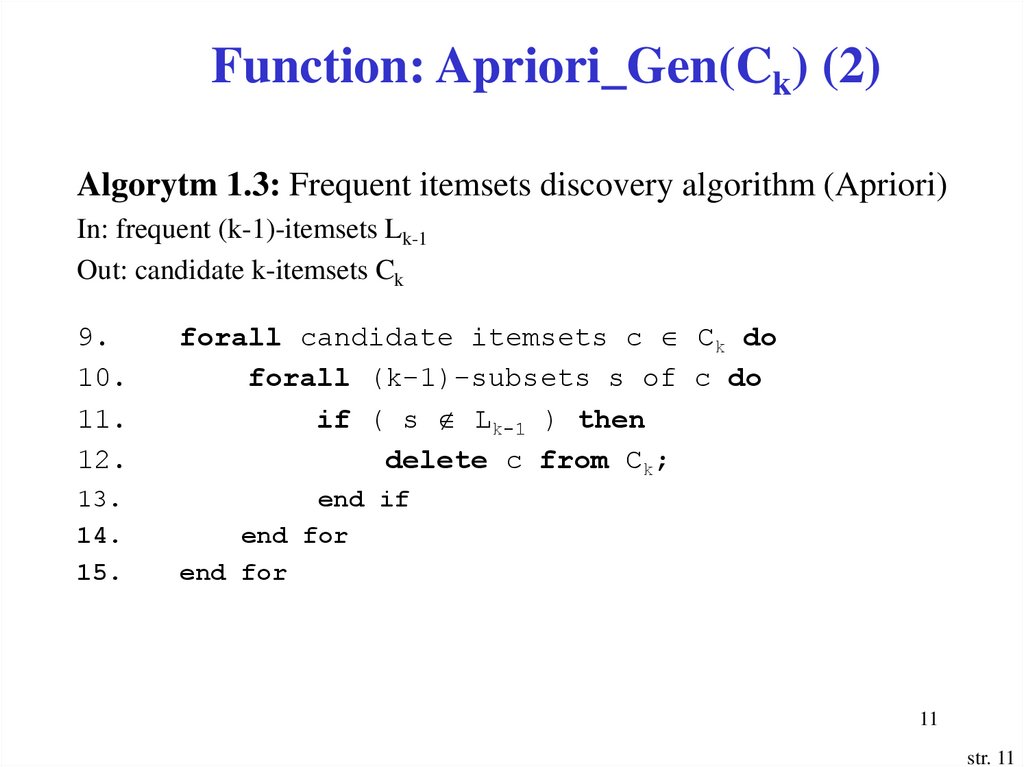
Function: Apriori_Gen(Ck) (2)
Algorytm 1.3: Frequent itemsets discovery algorithm (Apriori)
In: frequent (k-1)-itemsets Lk-1
Out: candidate k-itemsets Ck
9.
10.
11.
12.
forall candidate itemsets c Ck do
forall (k-1)-subsets s of c do
if ( s Lk-1 ) then
delete c from Ck;
13.
14.
15.
end if
end for
end for
11
str. 11

12. Example 2

• Assume that minsup = 50% (2 transactions)
TID Items
100
200
300
400
134
235
1235
25
C1
L1
Itemset Sup
Itemset
Sup
1
2
3
5
2
3
3
3
1
2
3
4
5
2
3
3
1
3
12

13. Example 2 (cont.)

C2
L2
itemset Sup
itemset
Sup
13
23
25
35
2
2
3
2
12
13
15
23
25
35
1
2
1
2
3
2
C3
L3
itemset Sup
itemset Sup
235
C4 =
2
235
2
L4 =
13

14. Apriori Candidate Generation (1)

• Given Lk, generate Ck+1 in two steps:
L2
itemset sup
13
23
25
35
2
2
3
2
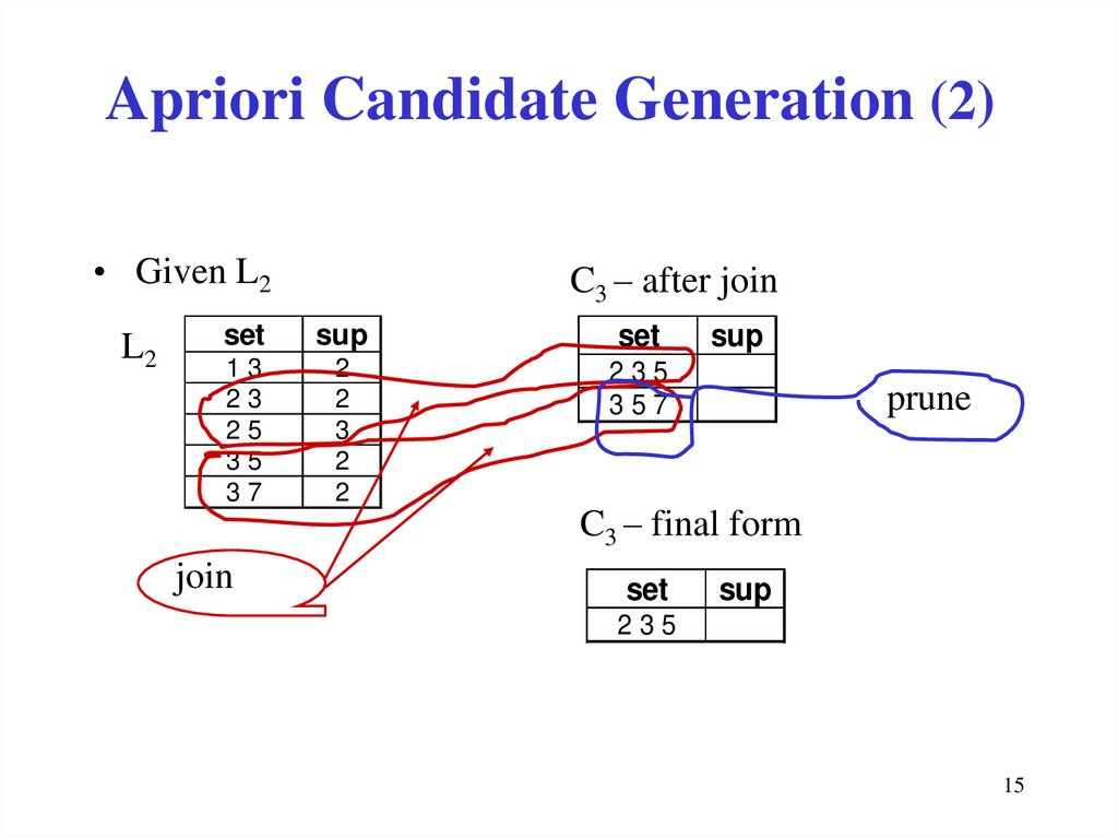
1. Join step: Join Lk1 with Lk2, with the join
condition that the first k-1 items should be the
same and Lk1[k] < Lk2[k]
2. Prune step: delete all candidates, which have a
non-frequent subset
14

15.

Apriori Candidate Generation (2)
• Given L2
L2
C3 – after join
set
sup
set
13
23
25
35
37
2
2
3
2
2
235
357
join
sup
prune
C3 – final form
set
sup
235
15

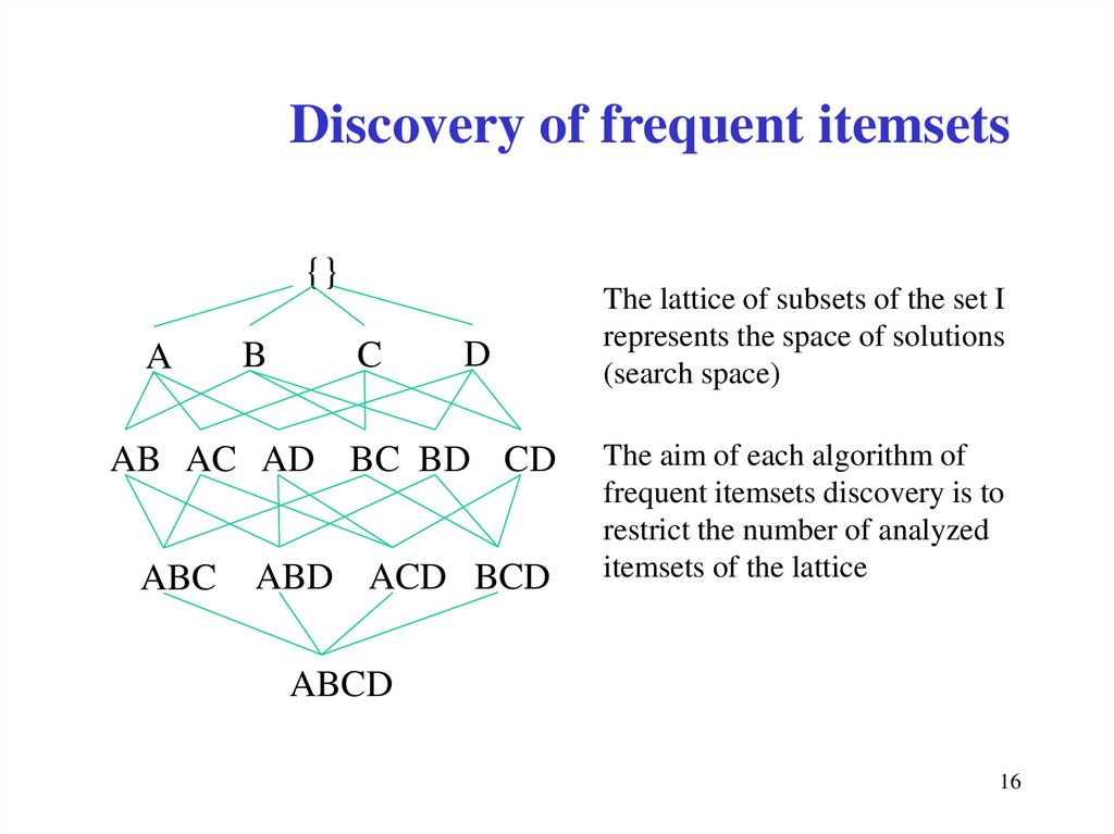
16.

Discovery of frequent itemsets
{}
A
B
C
D
AB AC AD BC BD CD
ABC
ABD ACD BCD
The lattice of subsets of the set I
represents the space of solutions
(search space)
The aim of each algorithm of
frequent itemsets discovery is to
restrict the number of analyzed
itemsets of the lattice
ABCD
16

17.

Properties of measures
Monotonicity property
Let I be a set of items, and J = 2|I| be the power set of I. A measure f is
monotone on the set J if:
X; Y J : (X Y) f (X) f (Y)
Monotone property of the measure f means that if X is a subset of
Y, then f (X) must not exceed f (Y)
Anti-monotonicity property
Let I be a set of items, and J = 2|I| be the power set of I. A measure f is
anti-monotone on the set J if:
X; Y J : (X Y) f (Y) f (X)
Anti-monotone property of the measure f means that if X is a subset of
Y, then f (Y) must not exceed f (X)
17
str. 17

18. Why does it work? (1)

• Anti-monotone property of the support measure:
all subsets of a frequent itemset are frequent, in
other words, if B is frequent and A B, then A is
also frequent
• Consequence: if A is not frequent, then it is not
necessary to generate the itemsets which include A
18

19. Apriori Property

not frequent
A
AB
ABC
B
AC
AD
ABD
ABCD
C
D
BC
BD
ACD
CD
BCD
not frequent, too
19

20. Why does it work? (2)

• The join step is equivalent to extending each
itemset in Lk with every item in the database and
then deleting those itemsets Ck+1 whose subset
(Ck+1 –C[k]) is not frequent.
20

21. Discovering Rules

L3
itemset sup
235
23 5
25 3
35 2
2 35
3 25
5 23
2
support = 2
support = 2
support = 2
support = 2
support = 2
support = 2
confidence = 100%
confidence = 66%
confidence = 100%
confidence = 66%
confidence = 66%
confidence = 66%
21

22. Rule generation (1)

• For each k-itemset X we can produce up
to 2k – 2 association rules
• Confidence does not have any monotone property
• conf(X Y) ??? conf(X’ Y’),
where X’ X and Y’ Y
• Is it possibble to prune association rules using the
confidence measure?
22

23. Rule generation (2)

• Given a frequent iteset Y
• Theorem:
if a rule X Y – X does not satisfy the minconf
threshold, then any rule X’ Y – X’, where X’
X, must not satisfy the minconf threshold as well
• Prove the theorem
23

24. Rule generation (3)

low-confidence
rule
b, c, d a
c, d a, b
b, d a, c
d a, b, c
a, b, c, d {}
a, c, d b
a, b, d c
b, c a, d
a, d b, c
c a, b, d
b a, c, d
low-confidence
rule
a, b, c d
a, c b, d
a, b c, d
a b, c, d
24

25. Example 2

Given the following database:
TrID
product
1
2
3
4
5
bread, milk
beer, milk, sugar
bread
bread, beer, milk
beer, milk, sugar
Assume the following values for minsup and minconf:
minsup = 30%
minconf = 70%
25

26. Example 2 (cont.)

C1
L1
candidate 1-itemset
bread
milk
beer
sugar
id sup (%)
1
2
3
4
frequent 1-itemset
60
80
60
40
bread
milk
beer
sugar
id sup (%)
1
2
3
4
60
80
60
40
C2
L2
candidate 2-itemset sup (%)
frequent 2-itemset
sup (%)
12
23
24
34
40
60
40
40
12
13
14
23
24
34
40
20
0
60
40
40
26

27. Example 2 (cont.)

C3
L3
candidate 3-itemset sup (%)
frequent 3-itemset
sup (%)
234
40
234
C4 =
40
L4 =
This is the end of the first step - generation of frequent itemsets
27

28. Example 2 (cont.) rule generation

fi
1
1
2
2
3
3
4
4
5
5
5
5
5
5
sup
0.40
0.40
0.60
0.60
0.40
0.40
0.40
0.40
0.40
0.40
0.40
0.40
0.40
0.40
rule
beer sugar
sugar beer
beer milk
milk beer
sugar milk
milk sugar
milk bread
bread milk
beer sugar milk
beer milk sugar
sugar milk beer
beer sugar milk
sugar beer milk
milk beer sugar
conf
0.67
1.00
1.00
0.75
1.00
0.50
0.50
0.67
1.00
0.67
1.00
0.67
1.00
0.50
28

29. Example 2 (cont.) rule generation

Only few rules fulfil the confidence requirements.
So, the final result of Apriori algorithm is the
following:
fi
1
2
2
3
5
5
5
sup
0.40
0.60
0.60
0.40
0.40
0.40
0.40
rule
sugar beer
beer milk
milk beer
sugar milk
beer sugar milk
sugar milk beer
sugar beer milk
conf
1.00
1.00
0.75
1.00
1.00
1.00
1.00
29

30.

Closed frequent itemsets (1)
• In any large dataset we can discover millions of frequent itemsets
which has usually to be preserved for the future mining and rule
generation
• It is useful to identify a small representative set of itemsets from
which all other frequent itemsets can be derived
• Two such representations from which all other frequent itemsets
can be derived are closed frequent itemsets and maximal frequent
itemsets
30
str. 30

31.

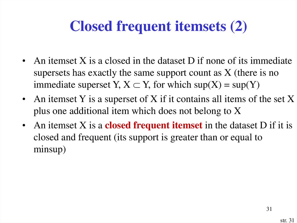
Closed frequent itemsets (2)
• An itemset X is a closed in the dataset D if none of its immediate
supersets has exactly the same support count as X (there is no
immediate superset Y, X Y, for which sup(X) = sup(Y)
• An itemset Y is a superset of X if it contains all items of the set X
plus one additional item which does not belong to X
• An itemset X is a closed frequent itemset in the dataset D if it is
closed and frequent (its support is greater than or equal to
minsup)
31
str. 31

32.

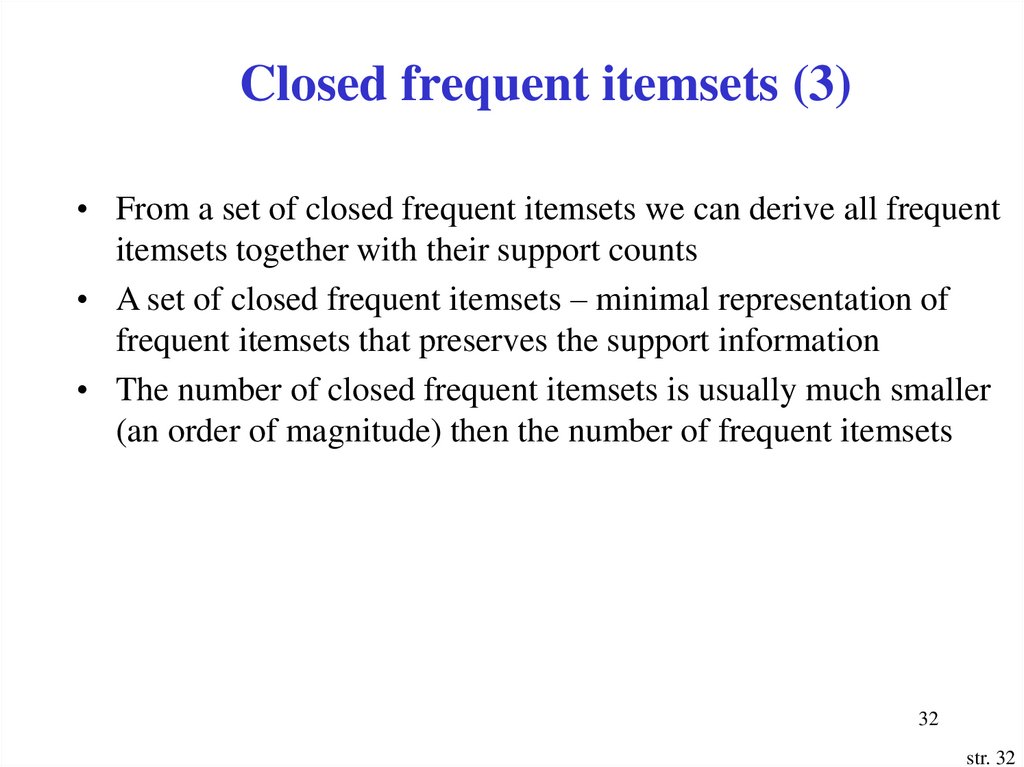
Closed frequent itemsets (3)
• From a set of closed frequent itemsets we can derive all frequent
itemsets together with their support counts
• A set of closed frequent itemsets – minimal representation of
frequent itemsets that preserves the support information
• The number of closed frequent itemsets is usually much smaller
(an order of magnitude) then the number of frequent itemsets
32
str. 32

33.

Closed frequent itemsets (4)
dataset
tid
1
2
3
4
5
items
A, B
B, C, D
A
A, B, D
B, C, D
Assume that the
minimum support
threshold minsup = 30%
(2 transactions)
set
A
B
C
D
A, B
A, C
A, D
B, C
B, D
C, D
A, B, C
A, B, D
A, C, D
B, C, D
A, B, C, D
support
3
4
2
3
2
0
1
2
3
2
0
1
0
2
0
33
str. 33

34.

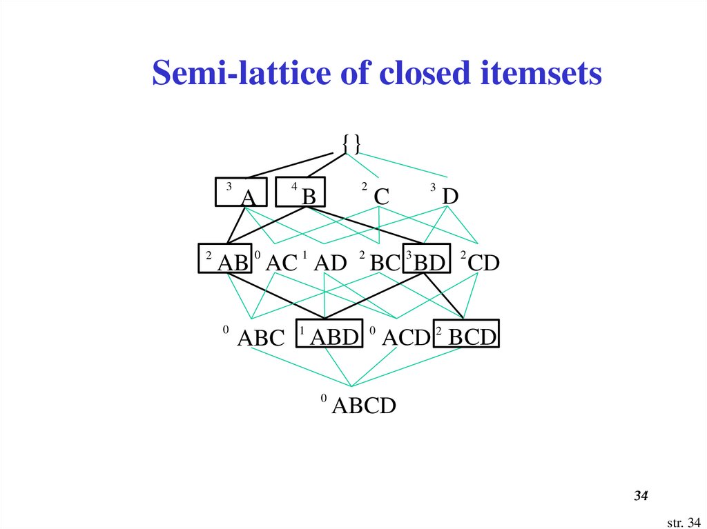
Semi-lattice of closed itemsets
{}
3
2
A
4
2
B
C
3
D
AB 0 AC 1 AD 2 BC 3 BD 2 CD
0
ABC 1 ABD 0 ACD 2 BCD
0
ABCD
34
str. 34

35.

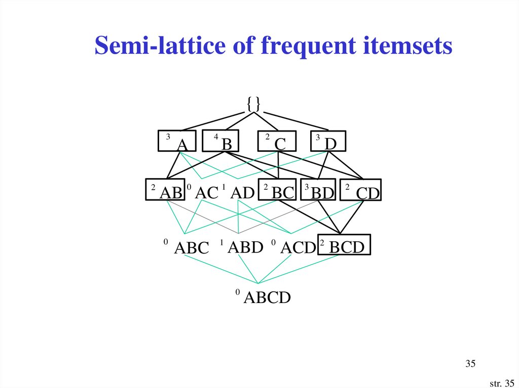
Semi-lattice of frequent itemsets
{}
3
2
A
4
2
B
C
3
D
AB 0 AC 1 AD 2 BC 3 BD 2 CD
0
ABC 1 ABD 0 ACD 2 BCD
0
ABCD
35
str. 35

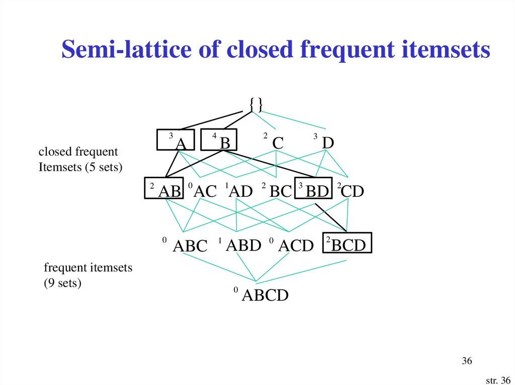
36.

Semi-lattice of closed frequent itemsets
{}
3
closed frequent
Itemsets (5 sets)
2
2
B
C
3
D
AB 0AC 1AD 2 BC 3 BD 2CD
0
frequent itemsets
(9 sets)
A
4
ABC
1
2
ABD 0 ACD BCD
0
ABCD
36
str. 36

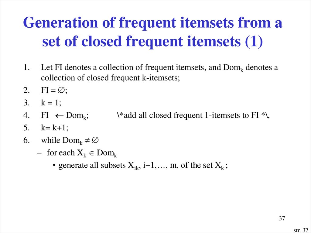
37.

Generation of frequent itemsets from a
set of closed frequent itemsets (1)
1.
2.
3.
4.
5.
6.
Let FI denotes a collection of frequent itemsets, and Domk denotes a
collection of closed frequent k-itemsets;
FI = ;
k = 1;
FI Domk;
\*add all closed frequent 1-itemsets to FI *\,
k= k+1;
while Domk
– for each Xk Domk
• generate all subsets Xik, i=1,…, m, of the set Xk ;
37
str. 37

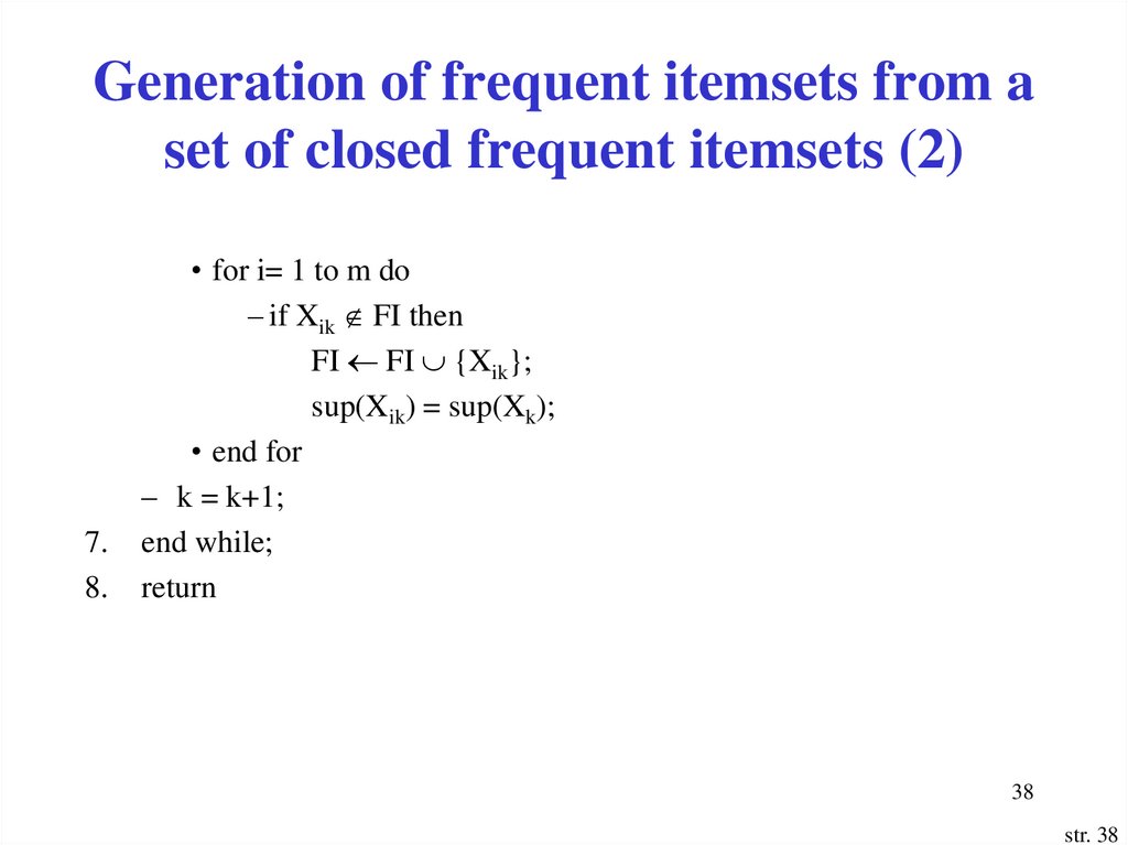
38.

Generation of frequent itemsets from a
set of closed frequent itemsets (2)
7.
8.
• for i= 1 to m do
– if Xik FI then
FI FI {Xik};
sup(Xik) = sup(Xk);
• end for
– k = k+1;
end while;
return
38
str. 38

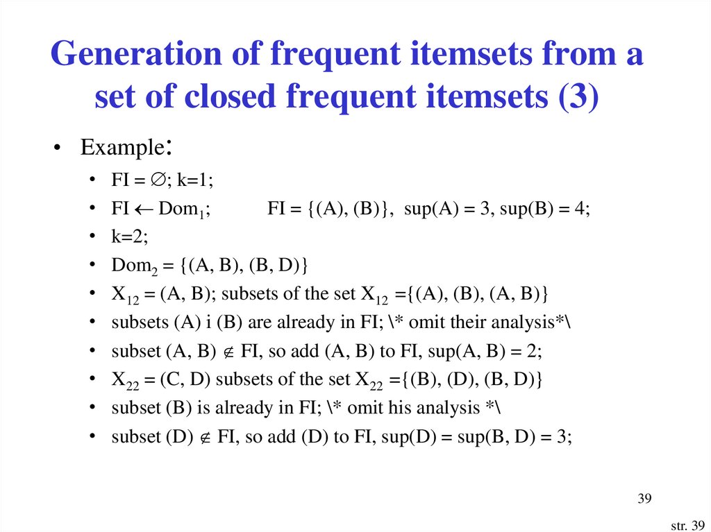
39.

Generation of frequent itemsets from a
set of closed frequent itemsets (3)
• Example:
FI = ; k=1;
FI Dom1;
FI = {(A), (B)}, sup(A) = 3, sup(B) = 4;
k=2;
Dom2 = {(A, B), (B, D)}
X12 = (A, B); subsets of the set X12 ={(A), (B), (A, B)}
subsets (A) i (B) are already in FI; \* omit their analysis*\
subset (A, B) FI, so add (A, B) to FI, sup(A, B) = 2;
X22 = (C, D) subsets of the set X22 ={(B), (D), (B, D)}
subset (B) is already in FI; \* omit his analysis *\
subset (D) FI, so add (D) to FI, sup(D) = sup(B, D) = 3;
39
str. 39

40.

Generation of frequent itemsets from a
set of closed frequent itemsets (4)
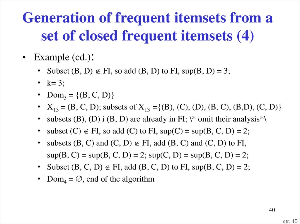
• Example (cd.):
Subset (B, D) FI, so add (B, D) to FI, sup(B, D) = 3;
k= 3;
Dom3 = {(B, C, D)}
X13 = (B, C, D); subsets of X13 ={(B), (C), (D), (B, C), (B,D), (C, D)}
subsets (B), (D) i (B, D) are already in FI; \* omit their analysis*\
subset (C) FI, so add (C) to FI, sup(C) = sup(B, C, D) = 2;
subsets (B, C) and (C, D) FI, add (B, C) and (C, D) to FI,
sup(B, C) = sup(B, C, D) = 2; sup(C, D) = sup(B, C, D) = 2;
• Subset (B, C, D) FI, add (B, C, D) to FI, sup(B, C, D) = 2;
• Dom4 = , end of the algorithm
40
str. 40

41.

Maximal frequent itemsets (1)
• An itemset X is a maximal frequent itemset in the dataset D if it
is frequent and none of its immediate supersets Y is frequent
• Maximal frequent itemsets provide most compact representation
of frequent itemsets, however they do contain the full support
information of their subsets
• All frequent itemsets contained in a dataset D are subsets of
maximal frequent itemsets of D
41
str. 41

42.

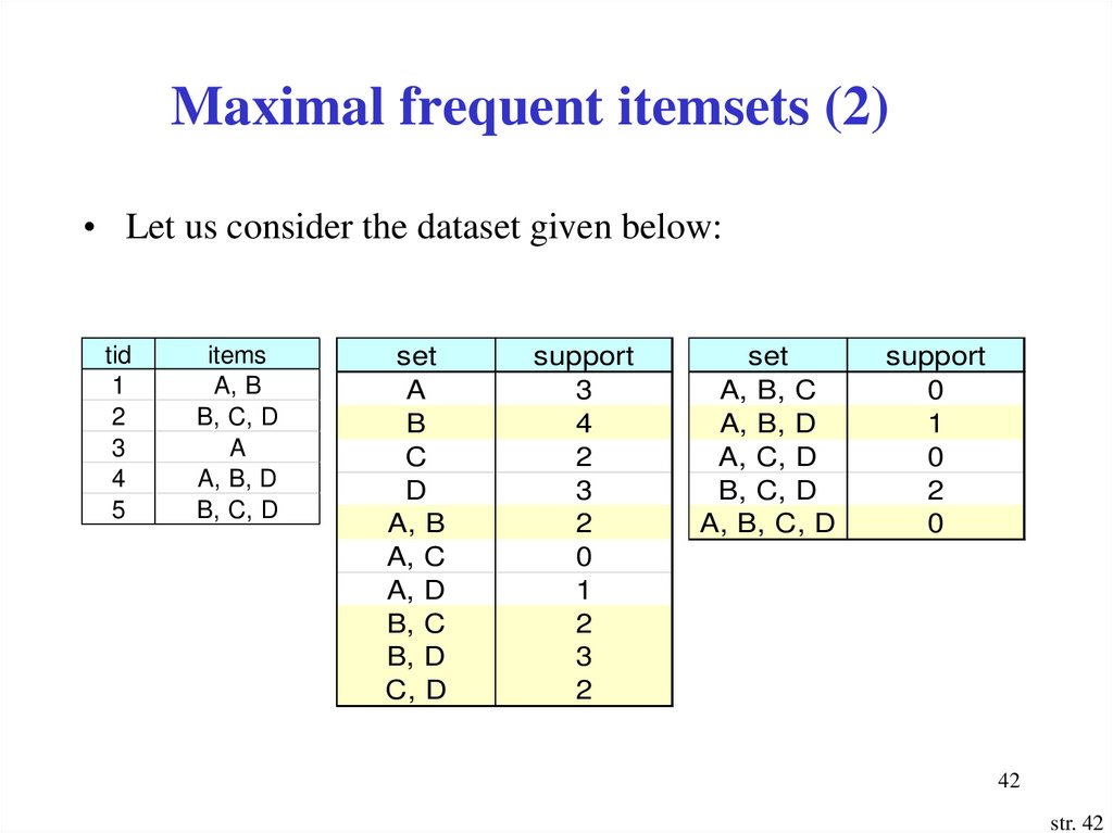
Maximal frequent itemsets (2)
• Let us consider the dataset given below:
tid
1
2
3
4
5
items
A, B
B, C, D
A
A, B, D
B, C, D
set
A
B
C
D
A, B
A, C
A, D
B, C
B, D
C, D
support
3
4
2
3
2
0
1
2
3
2
set
A, B, C
A, B, D
A, C, D
B, C, D
A, B, C, D
support
0
1
0
2
0
42
str. 42

43.

Maximal frequent itemsets (3)
{}
3
2
A
4
2
B
C
3
D
AB 0AC 1 AD 2 BC 3 BD 2 CD
0
ABC 1 ABD 0 ACD
0
2
BCD
ABCD
43
str. 43

44.

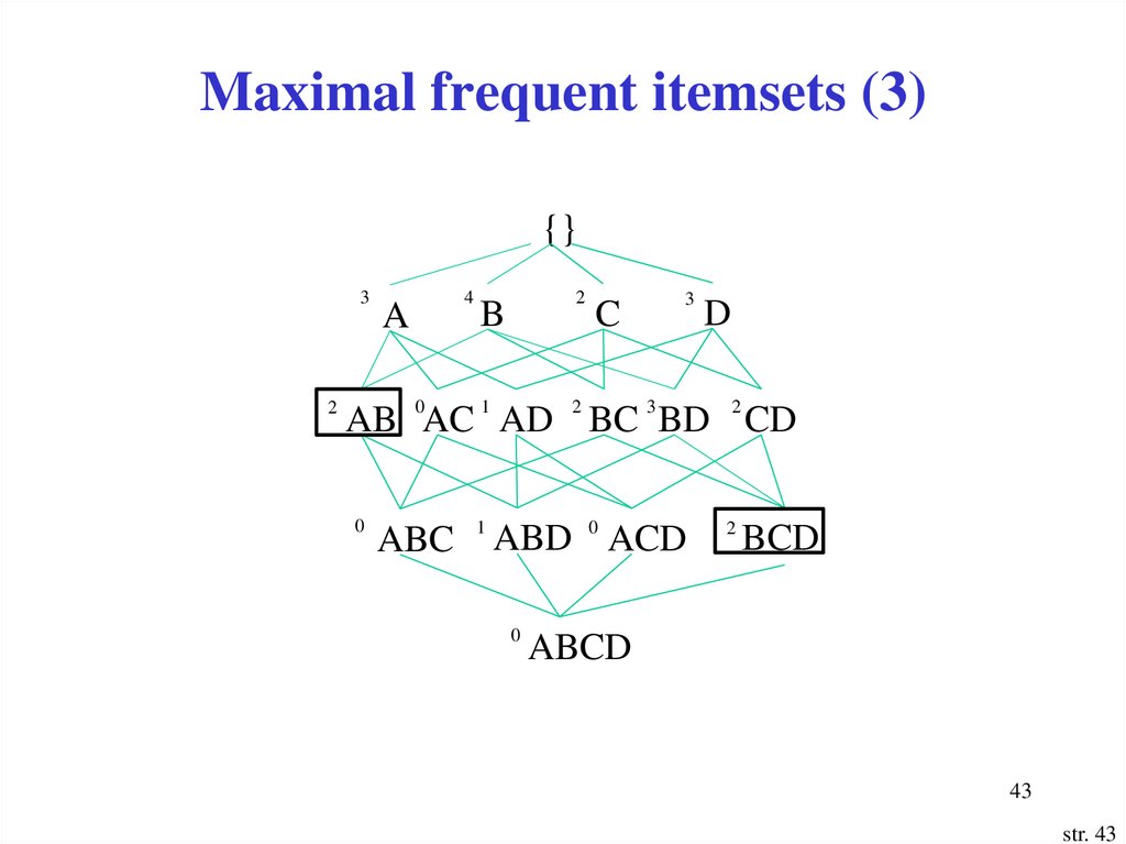
Maximal frequent itemsets (4)
• Maximal frequent itemsets:
(A, B) and (B, C, D)
• Easy to notice that all other frequent itemsets can be derived
from both sets
• From (A,B) the following 3 frequent itemsets can be derived:
(A), (B) i (A, B)
• From (B, C, D) we derive 6 frequent itemsets: (C), (D), (B, C),
(B, D), (C, D), (B, C, D)
• Maximal frequent itemsets provide most compact representation
of frequent itemsets, however they do contain the full support
information of their subsets
44
str. 44

45. Generalized Association Rules or Multilevel Association Rules

45

46. Multilevel AR (1)

• It is difficult to find interesting, strong
associations among data items at a too primitive
level due to the sparsity of data
• Approach: reason at suitable level of abstraction
• Data mining system should provide capabilities to
mine association rules at multiple levels of
abstractions and traverse easily among different
abstraction levels
46

47.

Multilevel AR (2)
• Multilevel association rule:
„50% of clients who purchase bread-stuff (bread, rolls,
purchase also diary products”
croissants, etc.)
• A multilevel (generalized) association rule is an association
rule which represents an association among named abstract
groups of items (events, properties, services, etc.)
• Multilevel association rules represent associations at multiple
levels of abstractions which are more understandable and
represent more general knowledge
• Multilevel association rules can’t be derived from single-level
association rules
47
str. 47

48. Multilevel AR - item hierarchy

• An attribute (item) may be generalized or specialized
according to a hierarchy of concepts (dimension
hierarchy!)
product
drink
juice
beer
breadstuff
clothes
wine
bread
shirts
outerwear
crescent
pants
jackets
48

49.

Item hierarchy
• Item hierarchy (dimension hierarchy) – semantic classification
of items
• It describes generalization/specialization relationship among items and/or
abstract groups of items
• It is a rooted tree whose leaves represent items of the set I, and whose
internal nodes represent abstract groups of items
• A root of the hierarchy represents the set I (all items)
• dimensions and levels can be efficiently encoded in transactions
• multilevel (generalized) association rules: rules which combine
associations with item hierarchy
49
str. 49

50. Basic algorithm (1)

1.
2.
3.
Extend each transaction Ti D by adding all ancestors
of each item in a transaction to the transaction (extended
transaction) (omit the root of the taxonomy and,
eventually, remove all repeating items)
Run any of algorithms for mining association rules over
those “extended transactions” (e.g. Apriori)
Remove all trivial multilevel association rules
50

51. Basic algorithm (2)

• A trivial multilevel association rule is the rule of the form
„node ancestor (node)”, where node represents a single
item or an abstract group of items
Use taxonomy information to prune redundant or
uninteresting rules
• Replace many specialized rules with one general rule: e.g.
rules „bread drinks” and „croissant drinks” replace
with the rule „breadstuff drinks” (use taxonomy
information to perform the replacement)
51

52. Drawbacks of the basic algorithm

• Drawbacks of the approach:
The number of candidate itemsets is much
larger,
The size of the average candidate itemset is
much larger.
The number of database scans is larger
52

53. MAR: uniform support vs. reduced support

• Uniform support: the same minimum
support for all levels
– one minsup: no need to examine itemsets
containing any item whose ancestors do not
have minimum support
– minsup value:
• high: miss low level associations
• low: generate too many high level associations
53

54. MAR: uniform support vs. reduced support

• Reduced Support: reduced minimum support at
lower levels - different strategies possible
milk
[support = 10%]
2% milk
[support = 6%]
Skim milk
[support = 6%]
54

55. Basic MAR discovery algorithm with reduced minsup

Top-down greedy algorithm
• Step 1: find all frequent items (abstract groups of items) at
the highest level of the taxonomy (most abstract level)
• Step 2: find all frequent items at consecutive lower levels
of the taxonomy – till leaves of the taxonomy
• Step 3: find frequent itemsets containing frequent items
belonging to different levels of the taxonomy
55