K-means and scikit learn

1.

2.

K-means
• In its simplest form, the algorithmik considers nearest neighborsonly one
nearest neighbor - the point of the training set, the closestlocated to the point
for which we want to get a forecast.The prediction is the answer already
known for the given training pointset.
• mglearn.plots.plot_knn_classification(n_neighbors=1)

3.

K-means
• Here we have added three new data points, shown asstars. For each, we marked the
nearest point of the trainingset. The prediction that the one nearest neighbor
algorithm gives is −the label of this point (shown by the color of the
marker).Instead of taking into account only one nearest neighbor, wewe can
consider an arbitrary number (k) neighbors. Hence andthe name of the algorithmk
nearest neighbors. When weconsider more than one neighbor, to assign a label is
usedvote (voting). This means that for each point of the testset, we count the
number of neighbors belonging to class 0, andnumber of class 1 neighbors. We
then assigntest set point most frequently occurring class: otherIn other words, we
choose the class with the majority amongk nearest neighbors.

4.

K-means
• In[11]:
• mglearn.plots.plot_knn_classification(n_neighbors=3)

5.

K-means and scikit learn
• Now let's see how the algorithm can be appliedk nearest neighbors using scikit-learn. First, we
will shareour data on the training and test sets to evaluategeneralizing ability of the model,
• from sklearn.model_selection import train_test_split
• X, y = mglearn.datasets.make_forge()
• X_train, X_test, y_train, y_test = train_test_split(X, y, random_state=0)

6.

K-means and scikit learn
• Next, we import and create an instance object of the class by
settingparameters, for example, the number of neighbors that we will usefor
classification. In this case, we set it to 3:
• from sklearn.neighbors import KNeighborsClassifier
• clf = KNeighborsClassifier(n_neighbors=3)

7.

K-means and sklearn
• We then fit the classifier using the training set. ForKNeighborsClassifier
which means remembering a set of data, suchThus, we can calculate the
neighbors during the prediction:
• clf.fit(X_train, y_train)

8.

Predict
• To get the predictions for the test data, we call the methodpredict. For each point of
the test set, it calculates its closestneighbors in the training set and finds among
them the most frequentoccurring class:
• print("Прогнозы на тестовом наборе: {}".format(clf.predict(X_test)))
• Out[15]:
• Прогнозы на тестовом наборе: [1 0 1 0 1 0 0]

9.

Score
• In[16]:
• print("Правильность на тестовом наборе: {:.2f}".format(clf.score(X_test,
y_test)))
• Out[16]:
• Правильность на тестовом наборе: 0.86

10.

Boundaries
• Also, for two-dimensional datasets, we can showpredictions for all possible
test set points by placing inxy plane. We will set the color of the plane
according to the classwhich will be assigned to a point in this area. This will
allow usformdecision boundary (decision boundary), whichsplits the plane
into two regions: the region where the algorithm assignsclass 0, and the
region where the algorithm assigns class 1.The code below renders the
bordersdecision making for one, three and nine neighbors

11.

Boundaries
In[17]:
fig, axes = plt.subplots(1, 3, figsize=(10, 3))
for n_neighbors, ax in zip([1, 3, 9], axes):
# создаем объект-классификатор и подгоняем в одной строке
clf = KNeighborsClassifier(n_neighbors=n_neighbors).fit(X, y)
mglearn.plots.plot_2d_separator(clf, X, fill=True, eps=0.5, ax=ax, alpha=.4)
mglearn.discrete_scatter(X[:, 0], X[:, 1], y, ax=ax)
ax.set_title("количество соседей:{}".format(n_neighbors))
ax.set_xlabel("признак 0")
ax.set_ylabel("признак 1")
axes[0].legend(loc=3)

12.

KNeighborsRegressor
• With regard to our one-dimensional data array, we cansee predictions for all
possible feature values (Figure 2.10).To do this, we create a test dataset and
visualizereceived forecast lines:

13.

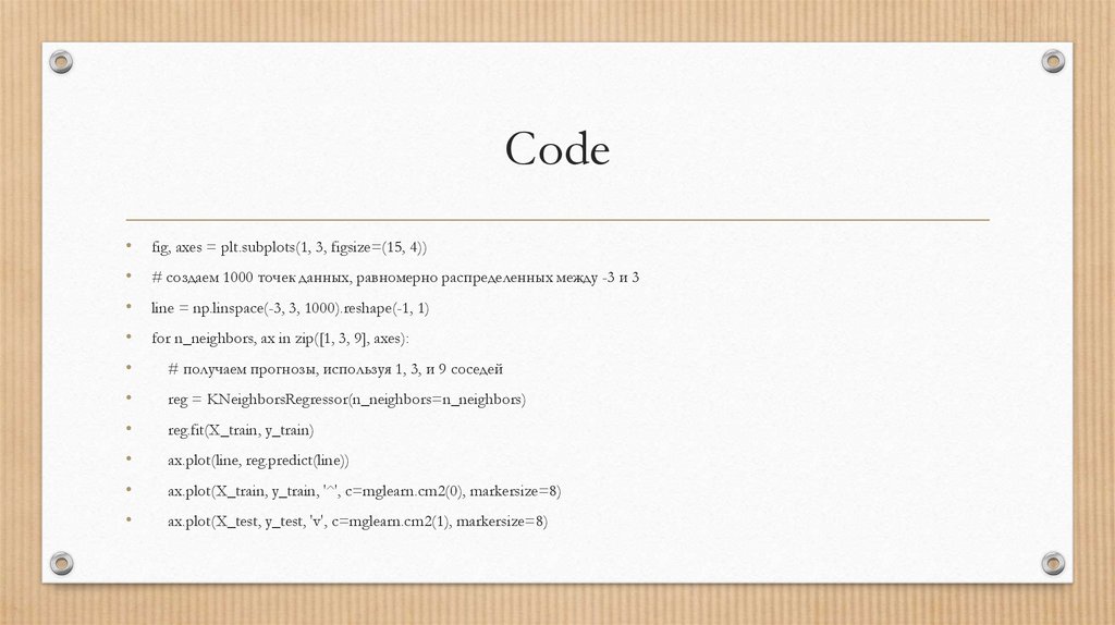
Code
fig, axes = plt.subplots(1, 3, figsize=(15, 4))
# создаем 1000 точек данных, равномерно распределенных между -3 и 3
line = np.linspace(-3, 3, 1000).reshape(-1, 1)
for n_neighbors, ax in zip([1, 3, 9], axes):
# получаем прогнозы, используя 1, 3, и 9 соседей
reg = KNeighborsRegressor(n_neighbors=n_neighbors)
reg.fit(X_train, y_train)
ax.plot(line, reg.predict(line))
ax.plot(X_train, y_train, '^', c=mglearn.cm2(0), markersize=8)
ax.plot(X_test, y_test, 'v', c=mglearn.cm2(1), markersize=8)

14.

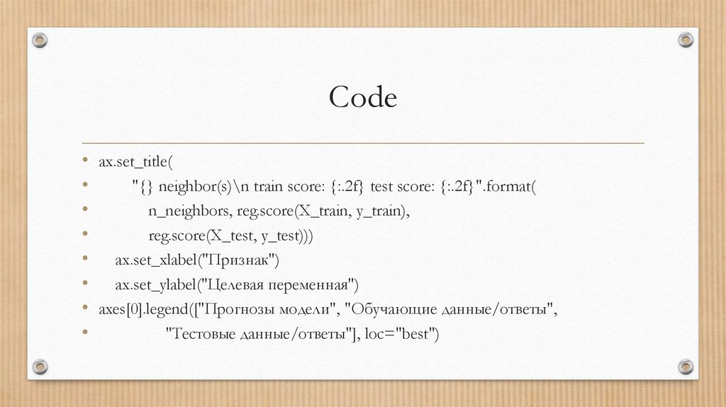
Code
• ax.set_title(
"{} neighbor(s)\n train score: {:.2f} test score: {:.2f}".format(
n_neighbors, reg.score(X_train, y_train),
reg.score(X_test, y_test)))
• ax.set_xlabel("Признак")
• ax.set_ylabel("Целевая переменная")
• axes[0].legend(["Прогнозы модели", "Обучающие данные/ответы",
"Тестовые данные/ответы"], loc="best")

15.

Advantages and disadvantages
• Basically, there are two important parameters in the KNeighbors classifier:the
number of neighbors and a measure of the distance between data points. On
thepractice, the use of a small number of neighbors (for example, 3-5) is
oftenworks well, but you can of course customize this one yourselfparameter. The
question of choosing the correct measure of distance,is outside the scope of this
book. The default is Euclideana distance that works well in many situations.One of
the advantages of the nearest neighbor method is thatthis model is very easy to
interpret and, as a rule, this method givesacceptable quality without the need for a
largenumber of settings.

16.

Advantages and disadvantages
• Typically, building a modelnearest neighbors happens very fast, but when
your trainingthe set is very large (in terms of the number of features
ornumber of observations) obtaining forecasts may take sometime. When
using the nearest neighbors algorithm, it is importantperform data
preprocessing (see chapter 3).This method does not work so well when it
comes to datasets.with a large number of signs (hundreds or more), and
especially badworks in a situation where the vast majority of features are
moreparts of the observations have zero values (the so-calledsparse datasets
orsparse datasets).

17.

Decision trees
• Building a decision tree means building a sequencerules "if ... then ...", which
leads us to the true answerin the shortest possible way. In machine learning,
these rulescalledtests (tests). Do not confuse them with the test set, whichwe
use to test the generalizing ability of our model.As a rule, data is presented
not only in the form of binaryyes/no signs, as in the example with animals,
but also in the form of continuousfeatures, as in the two-dimensional dataset
shown in Fig. 2.23.Tests that are used for continuous data are of the
form"Sign i more value a?"

18.

Decision trees
• mglearn.plots.plot_tree_progressive()

19.

Decision trees
• The recursive partitioning of the data is repeated until all pointsdata in each
split area (each leaf of the decision tree) is notwill belong to the same value
of the target variable(class or quantitative value). The leaf of the tree that
containsdata points referring to the same target valuevariable is calledclean
(pure). The final partition for ourdata set is shown in fig.

20.

Pruning
Let's take a closer look at how preflight works.clipping on the example of the
Breast Cancer dataset. As always, weimport the dataset and split it into training
and testparts. We then build the model using the default settings forbuilding a
complete tree (we grow a tree until allthe leaves will not become clean). Fix
random_state forreproducibility of results:

21.

Pruning
In[58]:
from sklearn.tree import DecisionTreeClassifier
cancer = load_breast_cancer()
X_train, X_test, y_train, y_test = train_test_split(
cancer.data, cancer.target, stratify=cancer.target, random_state=42)
tree = DecisionTreeClassifier(random_state=0)
tree.fit(X_train, y_train)
print("Правильность на обучающем наборе: {:.3f}".format(tree.score(X_train, y_train)))
print("Правильность на тестовом наборе: {:.3f}".format(tree.score(X_test, y_test)))
Out[58]:
Правильность на обучающем наборе: 1.000
Правильность на тестовом наборе: 0.937

22.

Pruning
• If you do not limit the depth, the tree can be arbitrarilydeep and complex.
Therefore, unpruned trees are prone toretraining and do not generalize well
to new data. Nowlet's apply a pre-pruning to the tree that will stopthe
process of building a tree before we perfectly fit the model totraining data.
One option is to stop the processbuilding a tree when a certain depth is
reached. We are hereset max_depth=4, that is, you can set only
foursequential questions (see Figures 2.24 and 2.26). Depth limittree reduces
overfitting. This leads to lowercorrectness on the training set, but improves
correctness ontest set:

23.

Pruning
In[59]:
tree = DecisionTreeClassifier(max_depth=4, random_state=0)
tree.fit(X_train, y_train)
print("Правильность на обучающем наборе: {:.3f}".format(tree.score(X_train, y_train)))
print("Правильность на тестовом наборе: {:.3f}".format(tree.score(X_test, y_test)))
Out[59]:
Правильность на обучающем наборе: 0.988
Правильность на тестовом наборе: 0.951

24.

Visualization
• from sklearn.tree import export_graphviz
• export_graphviz(tree, out_file="tree.dot", class_names=["malignant",
"benign"],
feature_names=cancer.feature_names, impurity=False,
filled=True)

25.

Visualization
• import graphviz
• with open("tree.dot") as f:
• dot_graph = f.read()
• graphviz.Source(dot_graph)

26.

Visualization
• import numpy as np
• import matplotlib.pyplot as plt
• import pandas as pd
• import mglearn
• %matplotlib inline
• from sklearn.model_selection import train_test_split
• from sklearn.datasets import load_breast_cancer

27.

Visualization
from sklearn import tree
from sklearn.tree import export_graphviz
cancer = load_breast_cancer()
X_train, X_test, y_train, y_test = train_test_split(
cancer.data, cancer.target, stratify=cancer.target, random_state=42)
clf = tree.DecisionTreeClassifier(max_depth=4, random_state=0)
clf = clf.fit(X_train, y_train)
import pydotplus
dot_data = tree.export_graphviz(clf, out_file=None)

28.

Ensembles
• Ensembles (ensembles) are methods that combine a set ofmachine learning
models to end up with a more powerfulmodel. There are many machine
learning models thatbelong to this category, but there are two ensemble
models thatproven to be effective on a wide variety of datasets
forclassification and regression problems, both use decision trees inas
building blocks: a random forest of decision trees and gradient boosting
decision trees.

29.

Random Forest
• As we have just noted, the main disadvantage of decision treesis their
tendency to overlearn. Random forest is oneof the ways to solve this
problem. Essentially, a random forest is a setdecision trees, where each tree is
slightly different from the others.The idea of a random forest is that each
tree canPretty good at predicting, but likely overfitting into piecesdata. If we
build many trees that work well andoverfitting to varying degrees, we can
reduce overfittingby averaging their results. Reduction of overfitting
atpreserving the predictive power of trees can be illustrated withusing
rigorous mathematics.

30.

Random forest
from sklearn.ensemble import RandomForestClassifier
from sklearn.datasets import make_moons
X, y = make_moons(n_samples=100, noise=0.25, random_state=3)
X_train, X_test, y_train, y_test = train_test_split(X, y, stratify=y,
random_state=42)
forest = RandomForestClassifier(n_estimators=5, random_state=2)
forest.fit(X_train, y_train)

31.

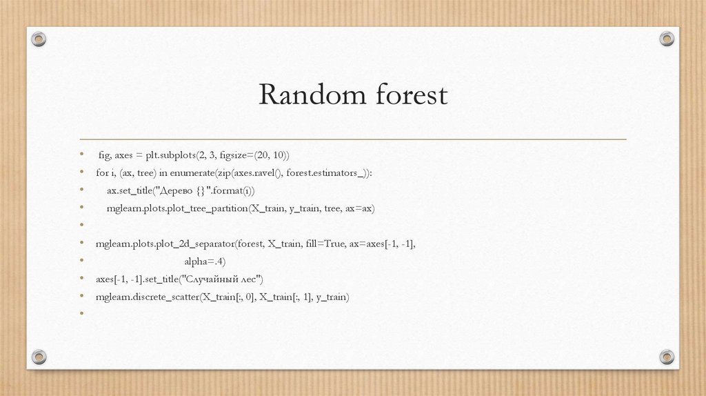
Random forest
fig, axes = plt.subplots(2, 3, figsize=(20, 10))
for i, (ax, tree) in enumerate(zip(axes.ravel(), forest.estimators_)):
ax.set_title("Дерево {}".format(i))
mglearn.plots.plot_tree_partition(X_train, y_train, tree, ax=ax)
mglearn.plots.plot_2d_separator(forest, X_train, fill=True, ax=axes[-1, -1],
alpha=.4)
axes[-1, -1].set_title("Случайный лес")
mglearn.discrete_scatter(X_train[:, 0], X_train[:, 1], y_train)

32.

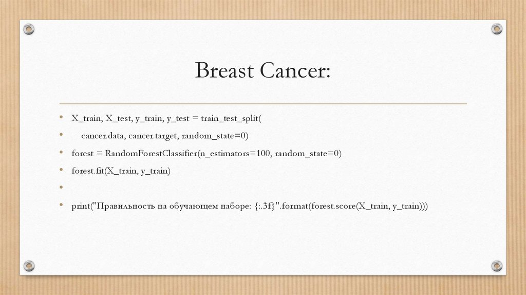
Breast Cancer:
• X_train, X_test, y_train, y_test = train_test_split(
cancer.data, cancer.target, random_state=0)
• forest = RandomForestClassifier(n_estimators=100, random_state=0)
• forest.fit(X_train, y_train)
• print("Правильность на обучающем наборе: {:.3f}".format(forest.score(X_train, y_train)))

33.

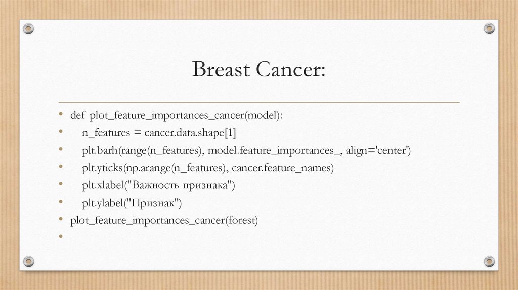
Breast Cancer:
• def plot_feature_importances_cancer(model):
• n_features = cancer.data.shape[1]
• plt.barh(range(n_features), model.feature_importances_, align='center')
• plt.yticks(np.arange(n_features), cancer.feature_names)
• plt.xlabel("Важность признака")
• plt.ylabel("Признак")
• plot_feature_importances_cancer(forest)

34.

Gradient Boosting
• The basic idea of gradient boosting is to combineset of simple models (in
this context known asnameweak students orweak learners), small
treesdepths. Each tree can only give good predictions for a part of it.data
and thus for iterative quality improvementmore and more trees are being
added.Gradient tree boosting often ranks first incompetitions in machine
learning, and is also widely used incommercial areas. Unlike random forest, it
usuallyslightly more sensitive to parameter settings, howevercorrectly set
parameters can give a higher valuecorrectness.

35.

Gradient Boosting
from sklearn.ensemble import GradientBoostingClassifier
X_train, X_test, y_train, y_test = train_test_split(
cancer.data, cancer.target, random_state=0)
gbrt = GradientBoostingClassifier(random_state=0)
gbrt.fit(X_train, y_train)
print("Правильность на обучающем наборе: {:.3f}".format(gbrt.score(X_train, y_train)))
print("Правильность на тестовом наборе: {:.3f}".format(gbrt.score(X_test, y_test)))

36.

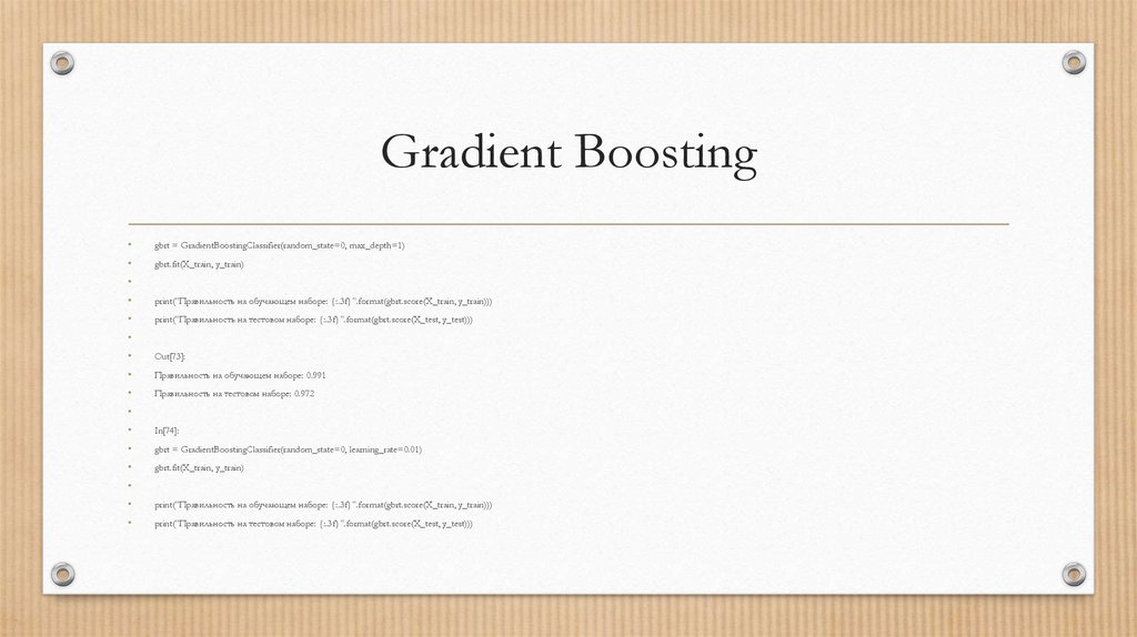
Gradient Boosting
gbrt = GradientBoostingClassifier(random_state=0, max_depth=1)
gbrt.fit(X_train, y_train)
print("Правильность на обучающем наборе: {:.3f}".format(gbrt.score(X_train, y_train)))
print("Правильность на тестовом наборе: {:.3f}".format(gbrt.score(X_test, y_test)))
Out[73]:
Правильность на обучающем наборе: 0.991
Правильность на тестовом наборе: 0.972
In[74]:
gbrt = GradientBoostingClassifier(random_state=0, learning_rate=0.01)
gbrt.fit(X_train, y_train)
print("Правильность на обучающем наборе: {:.3f}".format(gbrt.score(X_train, y_train)))
print("Правильность на тестовом наборе: {:.3f}".format(gbrt.score(X_test, y_test)))

37.

Visualization
gbrt = GradientBoostingClassifier(random_state=0, max_depth=1)
gbrt.fit(X_train, y_train)
def plot_feature_importances_cancer(model):
n_features = cancer.data.shape[1]
plt.barh(range(n_features), model.feature_importances_, align='center')
plt.yticks(np.arange(n_features), cancer.feature_names)
plt.xlabel("Важность признака")
plt.ylabel("Признак")
plot_feature_importances_cancer(gbrt)