


 programming
Similar presentations:


")

")


Machine Learning Algorithms. Lecture 1
1.
Machine Learning AlgorithmsDr. Leila Rzayeva
Lecture 1
Introduction in Machine Learning
2.
Course structure<30 hours of Oral Presentations
<20 hours Practice: homework/in-class assignments -> 60%
Final exam -> 40%
3.
Lab “Targets”• Weekly targets for your practical work
• Complete them on time!
• You’re an adult – manage your own time
• All material on Moodle
• It is an honor code violation to intentionally refer to other’s complete assignments
4.
Assignment- Work on assignments individually (!!!)
- Conduct a deep study of any topic in ML that you want!
(some suggestions will be provided)
- Produce a 3 page report
5.
Outline• Difference between AI and Machine Learning?
• Processes behind AI system
• Applications of AI & ML
• Basic Concepts of Machine Learning
• Rugby players and Ballet dancers example with Linear and Nearest
Neighbour classifiers
6.
ArtificialIntelligence
7.
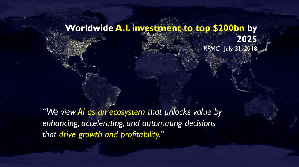
Worldwide A.I. investment to top $200bn by2025
KPMG. July 31, 2018
.
“We view AI as an ecosystem that unlocks value by
enhancing, accelerating, and automating decisions
that drive growth and profitability.”
8.
9.
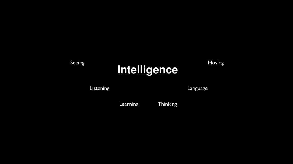
ArtificialIntelligence
10.
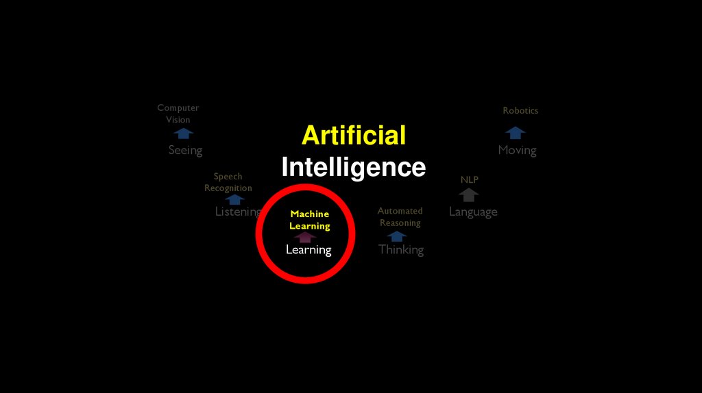
ArtificialIntelligence
Seeing
Listening
Moving
Language
Learning
Thinking
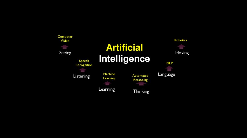
11.
ComputerVision
Robotics
Seeing
Speech
Recognition
Listening
Artificial
Intelligence
Machine
Learning
Learning
Automated
Reasoning
Thinking
Moving
NLP
Language
12.
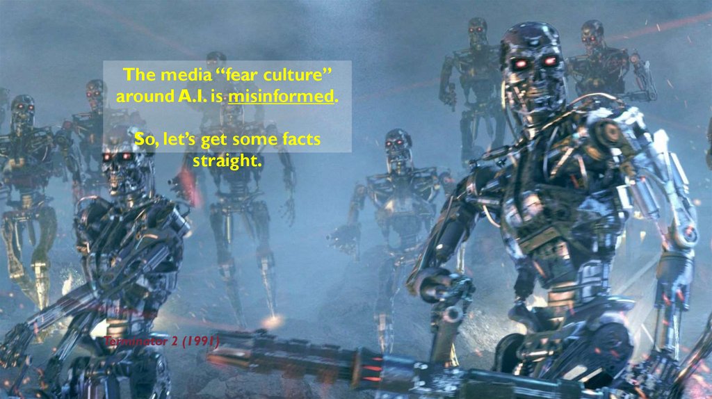
The media “fear culture”around A.I. is misinformed.
So, let’s get some facts
straight.
Terminator 2 (1991)
13.
“Strong”A.I. A.I.
“Strong”
...aims to build machines whose overall
intellectual ability is indistinguishable
from that of a human.
Ex Machina (2015)
14.
“Weak” A.I.…aims to engineer
commercially viable
"smart" systems
15.
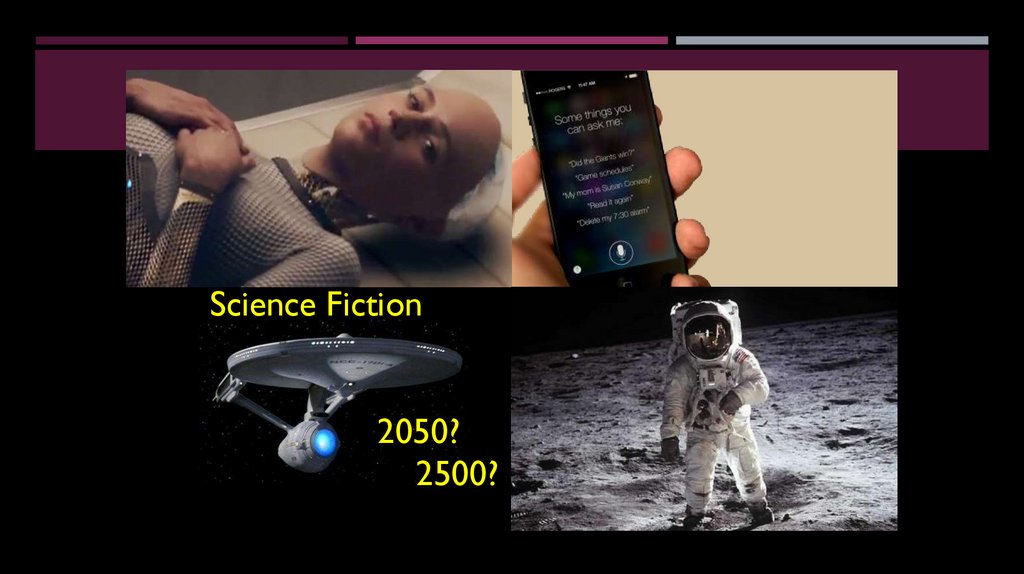
Science Fiction2050?
2500?
Science Fact
16.
17.
ComputerVision
Robotics
Seeing
Speech
Recognition
Listening
Artificial
Intelligence
Machine
Learning
Automated
Reasoning
Learning
Thinking
Moving
NLP
Language
18.
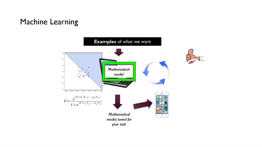
Machine LearningExamples of what we want
Mathematical
model
Probabilities, calculus,
linear algebra….
Mathematical
model, tuned for
your task
Human
“supervisor”
helps correct it
19.
20.
ComputerVision
Robotics
Seeing
Speech
Recognition
Listening
Artificial
Intelligence
Machine
Learning
Learning
Automated
Reasoning
Thinking
Moving
NLP
Language
21.
ComputerVision
Robotics
Seeing
Speech
Recognition
Listening
Artificial
Intelligence
Machine
Learning
Automated
Reasoning
Learning
Thinking
Moving
NLP
Language
22.
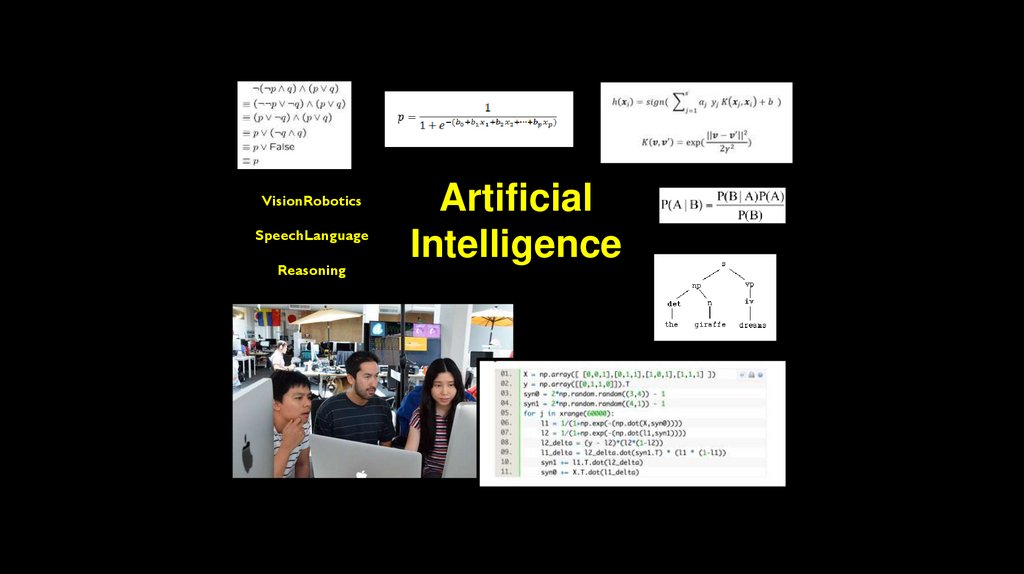
VisionRoboticsSpeechLanguage
Reasoning
Artificial
Intelligence
23.
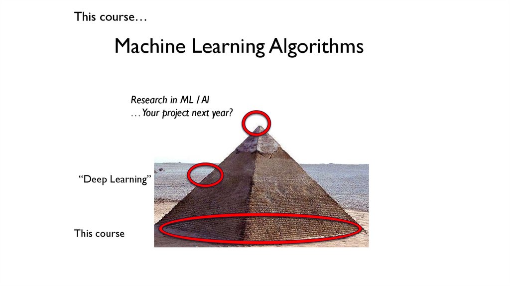
This course…Machine Learning Algorithms
Research in ML / AI
…Your project next year?
“Deep Learning”
This course
24.
Machine Learning25.
ComputerVision
Seeing
Artificial
Intelligence
Speech
Recognition
Listening
Robotics
Moving
NLP
Machine
Learning
Automated
Reasoning
Learning
Thinking
Language
26.
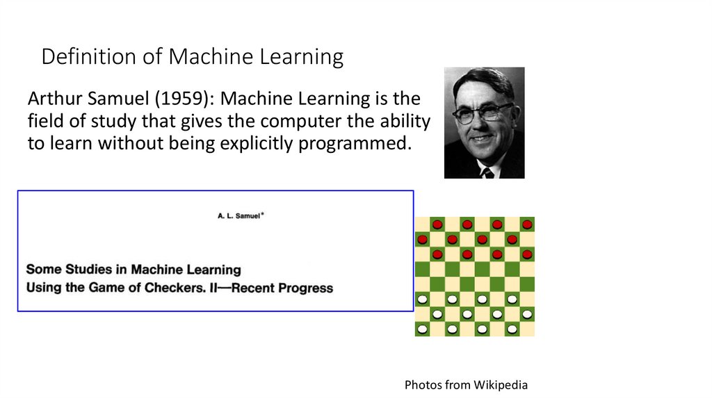
Definition of Machine LearningArthur Samuel (1959): Machine Learning is the
field of study that gives the computer the ability
to learn without being explicitly programmed.
Photos from Wikipedia
27.
DEFINITION OF MACHINELEARNING
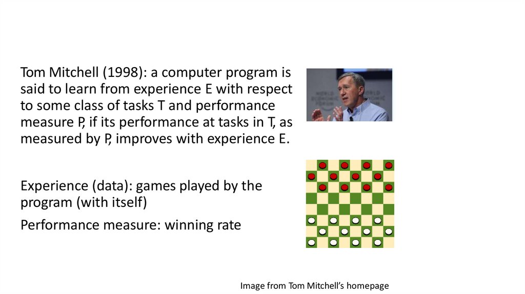
Tom Mitchell (1998): a computer program is
said to learn from experience E with respect
to some class of tasks T and performance
measure P, if its performance at tasks in T, as
measured by P, improves with experience E.
Experience (data): games played by the
program (with itself)
Performance measure: winning rate
Image from Tom Mitchell’s homepage
28.
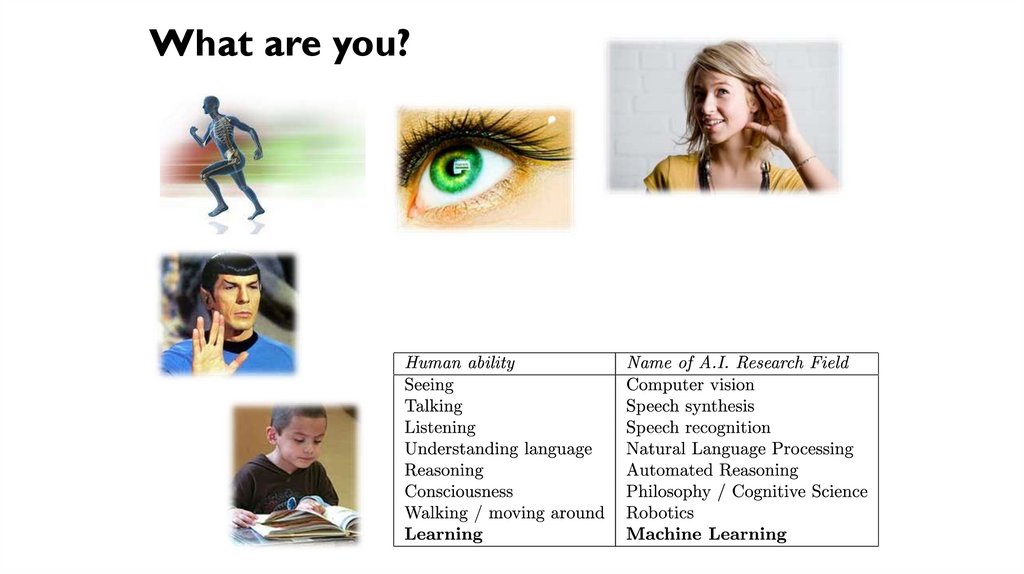
What are you?29.
“Learning” is a process- not specific to a substrate (e.g. biological neurons)
- can be mechanized, with a careful definition
30.
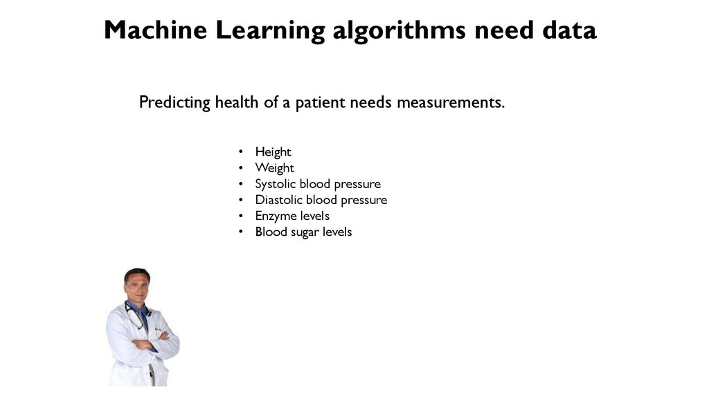
Machine Learning algorithms need dataPredicting health of a patient needs measurements.
Height
Weight
Systolic blood pressure
Diastolic blood pressure
Enzyme levels
Blood sugar levels
31.
Machine Learning algorithms need data“Examples”
height
70
23
56
50
12
56
…
…
…
…
56
weight
64
86
49
88
50
66
…
…
…
…
1
BP
3
5
5
3
1
2
…
…
…
…
5
enzyme
1
0
1
0
0
1
…
…
…
…
0
“Features”
Health?
1
1
0
0
1
0
…
…
…
…
0
Class, or “label”
Historical data in health records for example.
32.
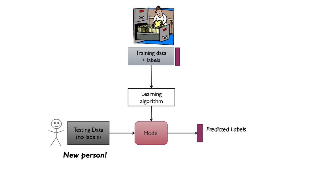
Training data+ labels
Learning
algorithm
Testing Data
(no labels)
New person!
Model
Predicted Labels
33.
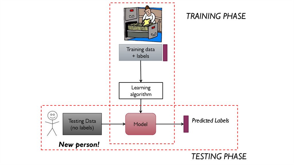
TRAINING PHASETraining data
+ labels
Learning
algorithm
Testing Data
(no labels)
Model
Predicted Labels
New person!
TESTING PHASE
34.
ML algorithms make mistakesPredicting health.
Quite a hard problem even for trained professional!
Next… Need to QUANTIFY performance of our algorithms.
Learning
algorithm
Model
35.
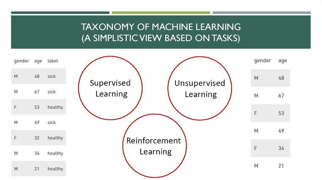
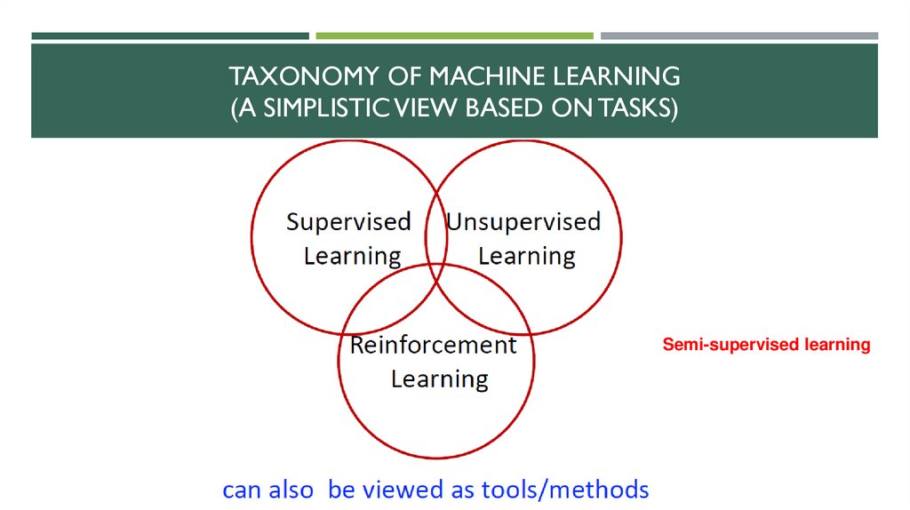
TAXONOMY OF MACHINE LEARNING(A SIMPLISTIC VIEW BASED ON TASKS)
36.
TAXONOMY OF MACHINE LEARNING(A SIMPLISTIC VIEW BASED ON TASKS)
Semi-supervised learning
37.
SUPERVISED LEARNING ALGORITHMS38.
EXAMPLE OF SUPERVISED LEARNING ALGORITHMS:Linear Regression
Logistic Regression
Nearest Neighbor
Gaussian Naive Bayes
Decision Trees
Support Vector Machine (SVM)
Random Forest
39.
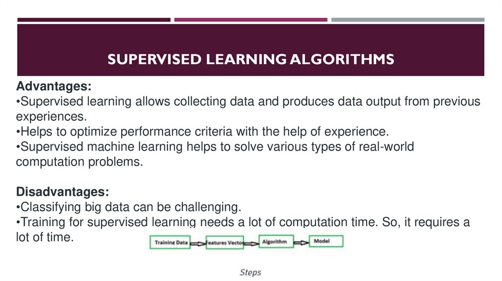
SUPERVISED LEARNING ALGORITHMSAdvantages:
•Supervised learning allows collecting data and produces data output from previous
experiences.
•Helps to optimize performance criteria with the help of experience.
•Supervised machine learning helps to solve various types of real-world
computation problems.
Disadvantages:
•Classifying big data can be challenging.
•Training for supervised learning needs a lot of computation time. So, it requires a
lot of time.
40.
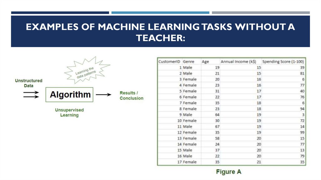
UNSUPERVISED LEARNING ALGORITHMSUnsupervised learning algorithms (unsupervised algorithms) are another type of algorithms. In unsupervised
learning algorithms, only objects are known, and there are no answers. Although there are many successful
applications of these methods, they tend to be more difficult to interpret and evaluate.
Examples of machine learning tasks without a teacher:
Identifying topics in a set of posts If you have a large collection of text data, you can aggregate them and find
common topics.You have no preliminary information about what topics are covered there and how many of them.
So there are no known answers.
41.
EXAMPLES OF MACHINE LEARNING TASKS WITHOUT ATEACHER:
42.
EXAMPLES OF MACHINE LEARNING TASKS WITHOUT ATEACHER:
43.
TYPES OF UNSUPERVISED LEARNING:44.
TYPES OF UNSUPERVISED LEARNING:Clustering
Exclusive (partitioning)
Agglomerative
Overlapping
Probabilistic
Clustering Types:
K-means clustering (DBSCAN, BIRCH)
Hierarchical clustering
Principal Component Analysis
Singular Value Decomposition
Independent Component Analysis
45.
MACHINE LEARNING TASKS WITHOUT A TEACHER:When solving machine learning tasks with and without a teacher, it is important to present your input data in a
format that is understandable to a computer.
Often the data is presented in the form of a table. Every data point you want to explore (every email, every
customer, every transaction) is a row, and every property that describes that data point (say, customer age, amount,
or transaction location) is a column. You can describe users by age, gender, account creation date and frequency of
purchases in your online store. You can describe the image of the tumor using grayscale for each pixel or using the
size, shape and color of the tumor.
46.
DISCUSS EXAMPLESIn machine learning, each object or row is called a sample or a data point, and the columns-properties that describe
these examples are called characteristics or features.
Later we will focus in more detail on the topic of data preparation, which is called feature extraction or feature
engineering. However, you should keep in mind that no machine learning algorithm will be able to make a
prediction based on data that does not contain any useful information.
For example, if the only sign of a patient is his last name, the algorithm will not be able to predict his gender. This
information is simply not in the data. If you add one more sign – the name of the patient, then things will already
be better, because often, knowing the name of a person, you can judge his gender.
47.
SEMI-SUPERVISED LEARNING:48.
Supervised vs. Unsupervised Machine Learning49.
REINFORCEMENT LEARNING ALGORITHMS50.
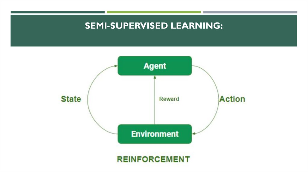
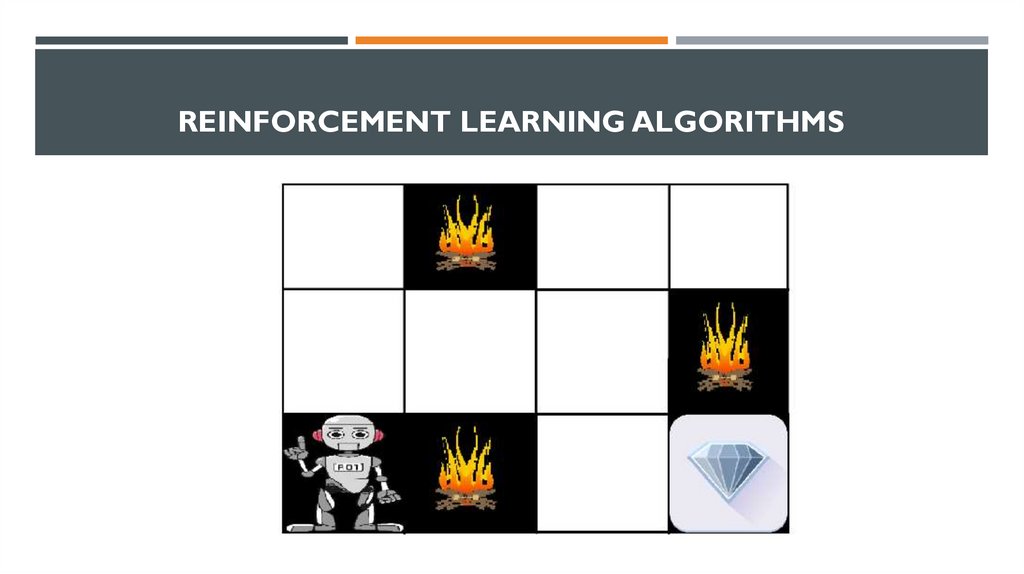
REINFORCEMENT LEARNING ALGORITHMSMain points in Reinforcement learning –
•Input: The input should be an initial state from which the model will start
•Output: There are many possible outputs as there are a variety of solutions to a
particular problem
•Training: The training is based upon the input, The model will return a state and
the user will decide to reward or punish the model based on its output.
•The model keeps continues to learn.
•The best solution is decided based on the maximum reward.
51.
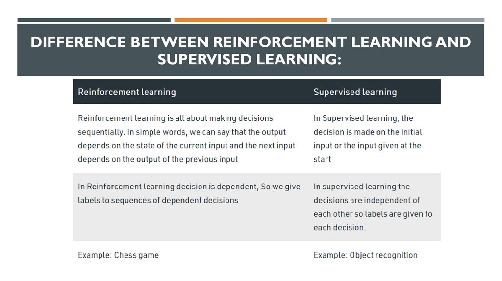
DIFFERENCE BETWEEN REINFORCEMENT LEARNING ANDSUPERVISED LEARNING:
52.
REINFORCEMENT LEARNING ALGORITHMSTypes of Reinforcement: There are two types of Reinforcement:
1. Positive –
Positive Reinforcement is defined as when an event, occurs due to a particular behavior, increases the
strength and the frequency of the behavior. In other words, it has a positive effect on
behavior.Advantages of reinforcement learning are:
• Maximizes Performance
• Sustain Change for a long period of time
• Too much Reinforcement can lead to an overload of states which can diminish the results
2. Negative –
Negative Reinforcement is defined as strengthening of behavior because a negative condition is stopped
or avoided.Advantages of reinforcement learning:
• Increases Behavior
• Provide defiance to a minimum standard of performance
• It Only provides enough to meet up the minimum behavior
53.
CATEGORIZING BASED ON REQUIRED OUTPUTAnother categorization of machine learning tasks arises when one considers the desired output of a machinelearned system:
1.Classification: When inputs are divided into two or more classes, the learner must produce a model that
assigns unseen inputs to one or more (multi-label classification) of these classes. This is typically tackled in a
supervised way. Spam filtering is an example of classification, where the inputs are email (or other) messages
and the classes are “spam” and “not spam”.
2.Regression: Which is also a supervised problem, A case when the outputs are continuous rather than discrete.
3.Clustering: When a set of inputs is to be divided into groups. Unlike in classification, the groups are not known
beforehand, making this typically an unsupervised task.
54.
DISCUSS EXAMPLES OF REINFORCEMENT LEARNINGVarious Practical applications of Reinforcement Learning –
•RL can be used in robotics for industrial automation.
•RL can be used in machine learning and data processing
•RL can be used to create training systems that provide custom instruction and materials
according to the requirement of students.
RL can be used in large environments in the following situations:
1.A model of the environment is known, but an analytic solution is not available;
2.Only a simulation model of the environment is given (the subject of simulation-based
optimization)
3.The only way to collect information about the environment is to interact with it.
55.
SCIENCE WITH PYTHONThe amount of digital data that exists is growing at a rapid rate, doubling every two years, and changing the way
we live. It is estimated that by 2020, about 1.7MB of new data will be created every second for every human being
on the planet. This means we need to have the technical tools, algorithms, and models to clean, process, and
understand the available data in its different forms for decision-making purposes.
Data science is the field that comprises everything related to cleaning, preparing, and analyzing unstructured,
semistructured, and structured data. This field of science uses a combination of statistics, mathematics,
programming, problem-solving, and data capture to extract insights and information from data.
56.
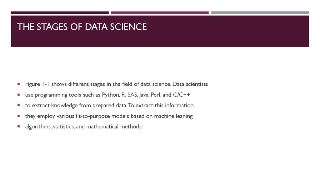
THE STAGES OF DATA SCIENCEFigure 1-1 shows different stages in the field of data science. Data scientists
use programming tools such as Python, R, SAS, Java, Perl, and C/C++
to extract knowledge from prepared data. To extract this information,
they employ various fit-to-purpose models based on machine leaning
algorithms, statistics, and mathematical methods.
57.
58.
WHY PYTHON?Python is a dynamic and general-purpose programming language that is used in various fields. Python is used for
everything from throwaway scripts to large, scalable web servers that provide uninterrupted service 24/7.
It is used for web programming, and application testing. It is used by scientists writing
applications for the world’s fastest supercomputers and by children first learning to program. It was initially
developed in the early 1990s by Guido van Rossum and is now controlled by the not-for-profit Python Software
Foundation, sponsored by Microsoft, Google, and others.
The first-ever version of Python was introduced in 1991. Python is now at version 3.x, which was released in
February 2011 after a long period of testing. Many of its major features have also been backported to the
backward-compatible Python 2.6, 2.7, and 3.6. GUI and database programming, client- and server-side
59.
BASIC FEATURES OF PYTHONPYTHON PROVIDES NUMEROUS FEATURES;
THE FOLLOWING ARE SOME OF THESE
IMPORTANT FEATURES:
• Easy to learn and use: Python uses an elegant syntax, making the programs easy to read. It is developer-friendly
and is a high-level programming language.
• Expressive: The Python language is expressive, which means it is more understandable and readable than other
languages.
• Interpreted: Python is an interpreted language. In other words, the interpreter executes the code line by line. This
makes debugging easy and thus suitable for beginners.
• Cross-platform: Python can run equally well on different platforms such as Windows, Linux, Unix, Macintosh, and
so on. So, Python is a portable language.
• Free and open source: The Python language is freely available at www.python.org. The source code is also
available.
60.
BASIC FEATURES OF PYTHONObject-oriented: Python is an object-oriented language with concepts of classes and objects.
• Extensible: It is easily extended by adding new modules implemented in a compiled language such as C or C++,
which can be used to compile the code.
• Large standard library: It comes with a large standard library that supports many common programming tasks
such as connecting to web servers, searching text with regular expressions, and reading and modifying files.
• GUI programming support: Graphical user interfaces can be developed using Python.
• Integrated: It can be easily integrated with languages such as C, C++, Java, and more.
61.
PORTABLE PYTHON EDITORS(NO INSTALLATION
REQUIRED)
These editors require no installation:
Azure Jupyter Notebooks: The open source Jupyter Notebooks was developed by Microsoft as an analytic
playground for analytics and machine learning.
Python(x,y): Python(x,y) is a free scientific and engineering development application for numerical computations,
data analysis, and data visualization based on the Python programming language, Qt graphical user interfaces,
and Spyder interactive scientific development environment.
WinPython: This is a free Python distribution for the Windows platform; it includes prebuilt packages for
ScientificPython.
Anaconda: This is a completely free enterprise ready Python distribution for large-scale data processing,
predictive analytics, and scientific computing.
62.
TABULAR DATA AND DATA FORMATSData is available in different forms. It can be unstructured data, semistructured data, or structured data.
Python provides different structures to maintain data and to manipulate it such as variables, lists, dictionaries,
tuples, series, panels, and data frames. Tabular data can be easily represented in Python using lists of tuples
representing the records of the data set in a data frame structure.
Though easy to create, these kinds of representations typically do not enable important tabular data
manipulations, such as efficient column selection, matrix mathematics, or spreadsheet-style operations. Tabular
is a package of Python modules for working with tabular data. Its main object is the tabarray class, which is a
data structure for holding and manipulating tabular data.You can put data into a tabarray object for more
flexible and powerful data processing.
The Pandas library also provides rich data structures and functions designed to make working with structured
data fast, easy, and expressive. In addition, it provides a powerful and productive data analysis environment.
A Pandas data frame can be created using the following constructor:
pandas.DataFrame( data, index, columns, dtype, copy)
63.
PANDAS DATA FRAMEA Pandas data frame can be created using various input forms such as the following:
List
Dictionary
Series
Numpy ndarrays
Another data frame
64.
PYTHON PANDAS DATA SCIENCE LIBRARYPandas is an open source Python library providing high-performance data manipulation and analysis tools via its
powerful data structures. The name Pandas is derived from “panel data,” an econometrics term from multidimensional
data. The following are the key features of the Pandas library:
Provides a mechanism to load data objects from different formats
Creates efficient data frame objects with default and customized indexing
Reshapes and pivots date sets
Provides efficient mechanisms to handle missing data
Merges, groups by, aggregates, and transforms data
Manipulates large data sets by implementing various functionalities such as slicing, indexing, subsetting, deletion, and
insertion
Provides efficient time series functionality
65.
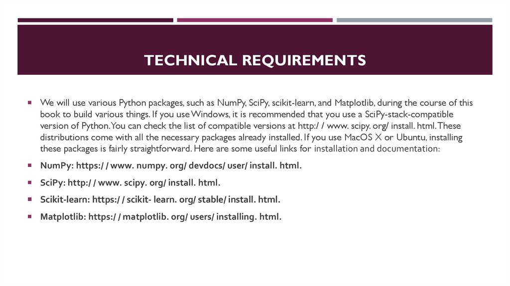
TECHNICAL REQUIREMENTSWe will use various Python packages, such as NumPy, SciPy, scikit-learn, and Matplotlib, during the course of this
book to build various things. If you use Windows, it is recommended that you use a SciPy-stack-compatible
version of Python.You can check the list of compatible versions at http:/ / www. scipy. org/ install. html. These
distributions come with all the necessary packages already installed. If you use MacOS X or Ubuntu, installing
these packages is fairly straightforward. Here are some useful links for installation and documentation:
NumPy: https:/ / www. numpy. org/ devdocs/ user/ install. html.
SciPy: http:/ / www. scipy. org/ install. html.
Scikit-learn: https:/ / scikit- learn. org/ stable/ install. html.
Matplotlib: https:/ / matplotlib. org/ users/ installing. html.
66.
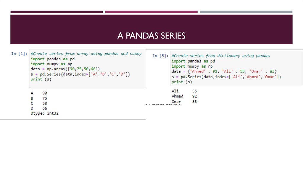
A PANDAS SERIESA series is a one-dimensional labeled array capable of holding data of any type (integer, string, float, Python objects,
etc.). Listing 1 shows how to create a series using the Pandas library.
67.
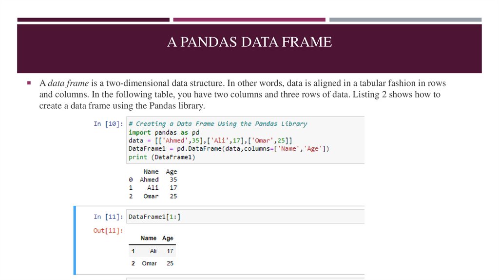
A PANDAS DATA FRAMEA data frame is a two-dimensional data structure. In other words, data is aligned in a tabular fashion in rows
and columns. In the following table, you have two columns and three rows of data. Listing 2 shows how to
create a data frame using the Pandas library.
68.
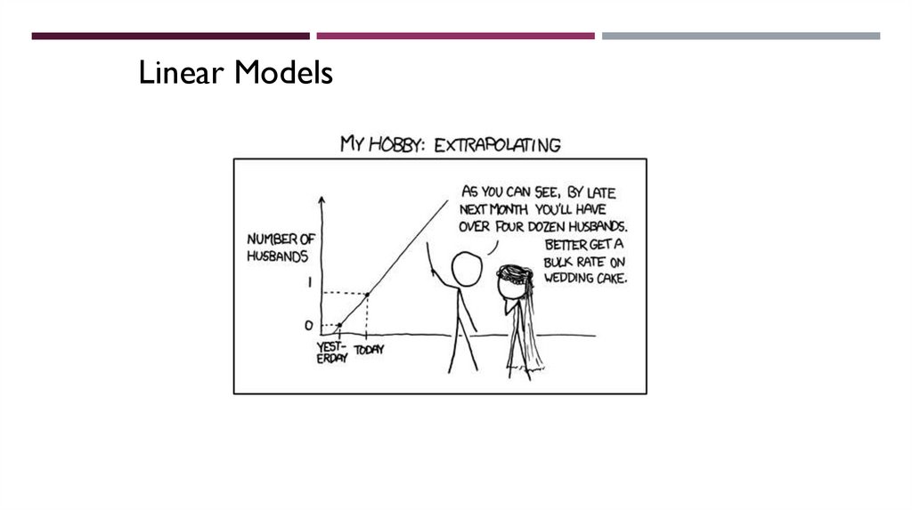
Linear Model69.
Linear Models70.
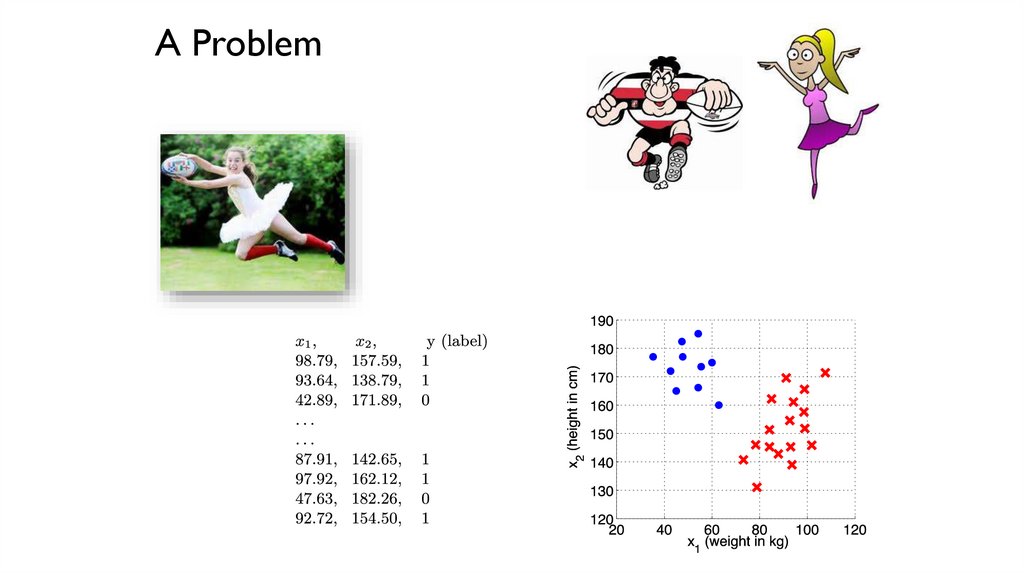
A Problem to Solve with Machine LearningDistinguish rugby players from ballet dancers.
You are provided with a few examples.
Almaty rugby club (16).
Astana ballet troupe (10).
Task
Generate a program which will correctly classify ANY player/dancer in the
world.
Hint
We shouldn’t “fine-tune” our system too much so it only works on the local clubs.
71.
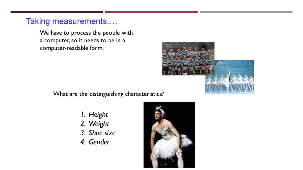
Taking measurements….We have to process the people with
a computer, so it needs to be in a
computer-readable form.
What are the distinguishing characteristics?
1. Height
2. Weight
3. Shoe size
4. Gender
72.
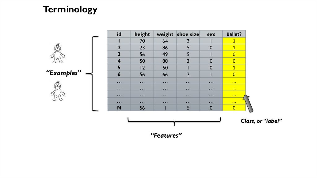
Terminology“Examples”
id
1
2
3
4
5
6
…
…
…
…
N
height
70
23
56
50
12
56
…
…
…
…
56
weight shoe size
3
64
86
5
49
5
88
3
50
1
66
2
…
…
…
…
…
…
…
…
1
5
sex
1
0
1
0
0
1
…
…
…
…
0
Ballet?
1
1
0
0
1
0
…
…
…
…
0
Class, or “label”
“Features”
73.
THE SUPERVISED LEARNING PIPELINETraining data
and labels
Learning algorithm
Testing Data
(no labels)
Model
Predicted Labels
74.
Taking measurements….Person
Weight
Height
1
2
3
4
5
…
16
17
18
19
20
…
63kg
55kg
75kg
50kg
57kg
…
85kg
93kg
75kg
99kg
100kg
…
190cm
185cm
202cm
180cm
174cm
150cm
145cm
130cm
163cm
171cm
75.
A Problem76.
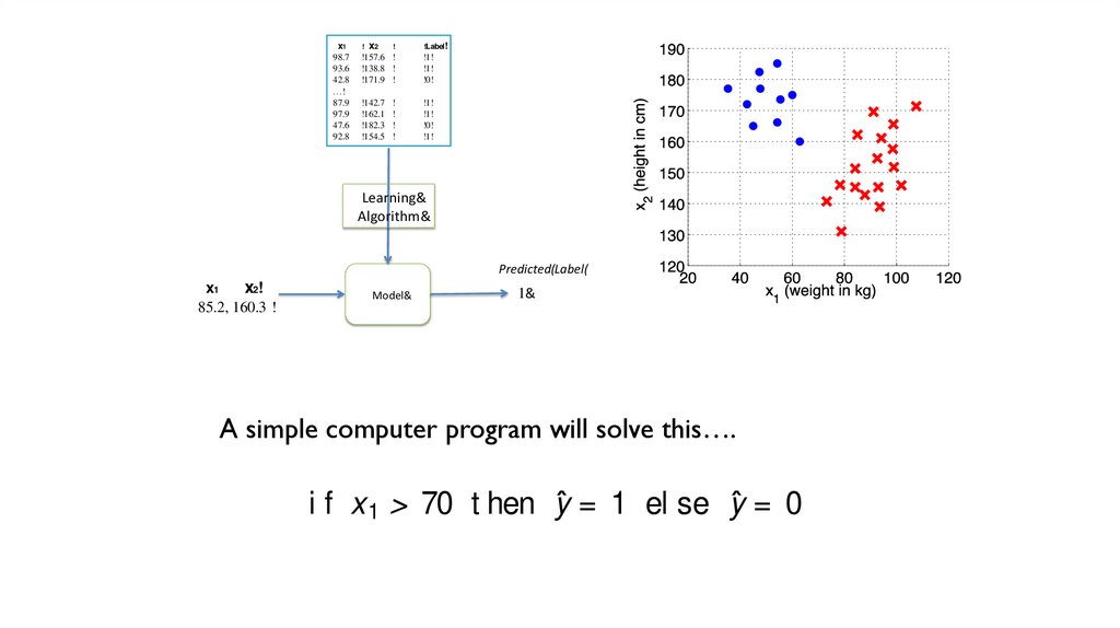
x = { 85.2, 160.3} .Figure 2.2: Reminder of the basic supervised learning pipeline — using training data to build a model, then evaluating it on unseen testing data. On this
course you will learn several di ↵erent model types, and the appropriate learning
algorithm for each.
x1
98.7
93.6
42.8
…!
87.9
97.9
47.6
92.8
! x2
!
!Label!
!157.6 !
!138.8 !
!171.9 !
!1!
!1!
!0!
!142.7
!162.1
!182.3
!154.5
!1!
!1!
!0!
!1!
!
!
!
!
Learning&
Algorithm&
2.1.2
Predicted(Label(
x
x!
T he
Simplest
L
inear
1&M odel: T he D ecision St ump
85.2, 160.3 !
1
2
Model&
Given a visualization of t he rugby-ballet dat a in gure 2.1, your own wellFigure 2.2: Reminder of the basic supervised learning pipeline — using trainengineered
learning
algorit
hmit on(i.e.
hat tdata.
hing
your ears) can spot a
ing data to build
a model, then
evaluating
unseent testing
On between
this
course you will learn several di ↵ erent model types, and the appropriate learning
pat tern.
can
writ ecomputer
a very simple
program
will solve t he problem,
A simple
program
will solvet hat
this….
algorithmWe
for each.
2.1.2
T he Sim plest Liinear
D ecision
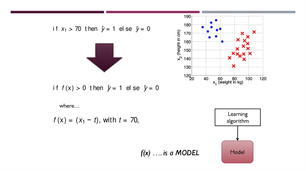
f x 1M>odel:
70 Tthehen
ŷ = St1umelp se
Given a visualizat ion of t he rugby-ballet dat a in gure 2.1, your own wellengineered learning algorit hm (i.e. t hat t hing between your ears) can spot a
pat t ern. We can writ e a very simple program t hat will solve t he problem,
ŷ = 0
(2.1)
where we use the not at ion ŷ to indicat e a predict ion of t he variable y. If we
imagine a funct ion f (x) = (x 1 − t), with t = 70, then an equivalent rule is:
77.
Givenof t he rugby-ballet
dat a it
in on
gure
2.1, your
owndata.
well- On this
ng
dataa visualization
to build a model,
then evaluating
unseen
testing
engineeredT learning
algorit hmL (i.e.
t hatMt hing
between
ears) canStspot
a
2.1.2
odel:
T he your
D ecision
ump
ourse
you he
will Simplest
learn
several inear
di ↵erent
model
types,
and
the
appropriate
learning
pat tern. We can writ e a very simple program t hat will solve t he problem,
lgorithm
for each. of the rugby-ballet dat a in gure 2.1, your own wellGiven
a visualization
engineered learning ialgorit
spot a
f x 1 >hm
70 (i.e.
t hen t hat
ŷ = t1hing
el sebetween
ŷ = 0 your ears) can(2.1)
pat t ern. We can write a very simple program t hat will solve the problem,
where we use the not at ion ŷ to indicat e a predict ion of t he variable y. If we
2.1.2
heion
Simplest
odel:
Tŷ he
Decision
ump
imagine aTfunct
f (x)
−Linear
t),t hen
with ŷt M
== 70,
then
equivalent
rule is: St(2.1)
i f =x (x>1 70
1 el
se an
=
0
1
Given
a visualization
of the
in
2.1, your
where we
use t he not
t he variable
y.
Ifown
we welli f atf ion
(x)
>ŷ 0t orugby-ballet
tindicat
hen ŷ e= a1 predict
eldata
se ŷion
= of
0 gure
(2.2)
ngineered
learning
algorithm
(i.e.with
that
between
your ears)
can spot a
magine a function
f (x)
= (x 1 − t),
t = thing
70, t hen
an equivalent
rule is:
The
pointWe
of can
writing
t hisain
t he simple
second way
is t hatthat
t he will
functsolve
ion f (x)
now
attern.
write
very
program
theisproblem,
self-contained, and we can now call it a model, in t hat it has a parameter, t. PA RAM ET ERS
i f f (x) > 0 t hen ŷ = 1 el se ŷ = 0
(2.2)
f xin
70second
t hen way
ŷ = is1 t hat
el se
= 0
1 >the
The point of writ ing it his
t heŷfunction
f (x) is now (2.1)
where…
self-cont
ained,
and
we
can
callindicate
it a m odel,
in that it ofhas
a paramet
RA M ET ERS
where we use the notat
ionnow
ŷ to
a prediction
the
variableer,y.t. IfPAwe
magine a function f (x) = (x 1 − t), with t = 70, then an equivalent rule is:
i f f (x) > 0 t hen ŷ = 1 el se ŷ = 0
Learning
algorithm
(2.2)
The point of writing this in the second way is that
theisfunction
f(x) ….
a MODELf (x) is nowModel
elf-contained, and we can now call it a model, in that it has a parameter, t. PARAMET ERS
78.
i f x 1 > 70 t hen ŷ = 1 el se ŷ = 0(2.1)
Given
a visualization
of the
rugby-ballet
in of gure
2.1, your
where we
use
t he “Decision
not at ion
ŷ t oStump”
indicat e aispredict
ion
t he variable
y. Ifown
we wellThe
adata
linear
model
engineered
learningf (x)
algorithm
(i.e.with
that
between
your ears)
can spot a
imagine a function
= (x 1 − t),
t = thing
70, t hen
an equivalent
rule is:
pattern. We can write a very simple program that will solve the problem,
i f f (x) > 0 t hen ŷ = 1 el se ŷ = 0
(2.2)
f xin
70second
t hen way
ŷ = is1 t hat
el se
= 0
1 >the
The point of writ ing it his
t heŷfunction
f (x) is now (2.1)
where…
self-cont
ained,
and
we
can
callindicate
it a m odel,
in that it of
has
a paramet
RA M ET ERS
where we use the notat
ionnow
ŷ to
a prediction
the
variableer,y.t. IfPAwe
imagine a function f (x) = (x 1 − t), with t = 70, then an equivalent rule is:
“Decision Boundary”
i f f (x) > 0 t hen ŷ = 1 el se ŷ = 0
(2.2)
The point of writing this in the second way is that the function f (x) is now
self-contained, and we can now call it a model, in that it has a parameter, t. PARAMET ERS
Learning
algorithm
Model
79.
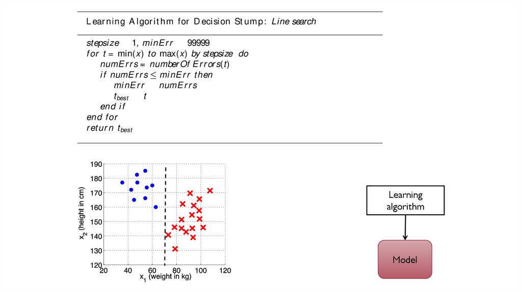
set t ing is what we refer t o as “ learning” .L ear ning A l gor i t hm for D eci sion St um p: Line search
stepsi ze 1, mi nE r r
99999
f or t = min(x) to max(x) by stepsize do
numE r r s = number Of E r r or s(t)
i f numE r r s mi nE r r t hen
mi nE r r
numE r r s
t best
t
end i f
end f or
r et ur n t best
Here, not e t hat we have assumed a funct ion number Of E r r or s(t) which evaluat es t he decision rule eq(2.2) wit h t hreshold t on t he dat a, and informs us how
many errors were made. Not ice also t hat we’ve had t o assume a stepsi ze, t he
Learning
algorithm
Model
80.
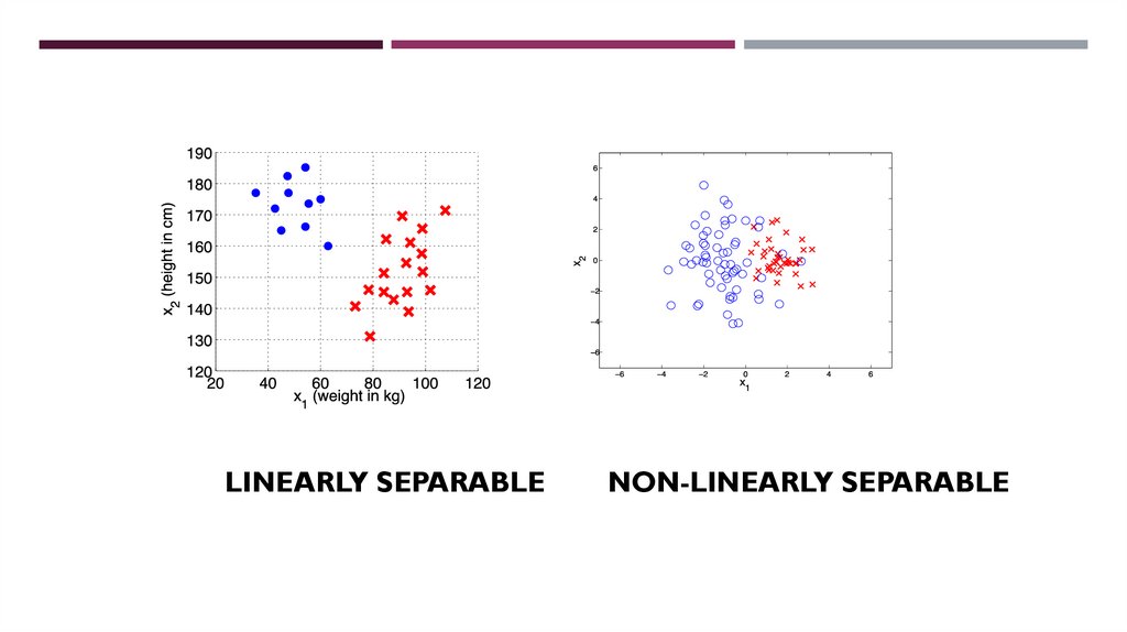
LINEARLY SEPARABLENON-LINEARLY SEPARABLE
81.
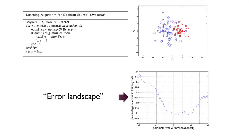
we do a simple line-search t o nd t he opt imal value, measuring t he number oferrors made on t he dat a for each possible t hreshold. Finding t he best paramet er
set t ing is what we refer t o as “ learning” .
L ear ning A l gor i t hm for D eci sion St um p: Line search
stepsi ze 1, mi nE r r
99999
f or t = min(x) to max(x) by stepsize do
numE r r s = number Of E r r or s(t)
i f numE r r s mi nE r r t hen
mi nE r r
numE r r s
t best
t
end i f
end f or
r et ur n t best
Here, not e t hat we have assumed a funct ion number Of E r r or s(t) which evaluat es t he decision rule eq(2.2) wit h t hreshold t on t he dat a, and informs us how
many errors were made. Not ice also t hat we’ve had t o assume a stepsi ze, t he
“Error landscape”
82.
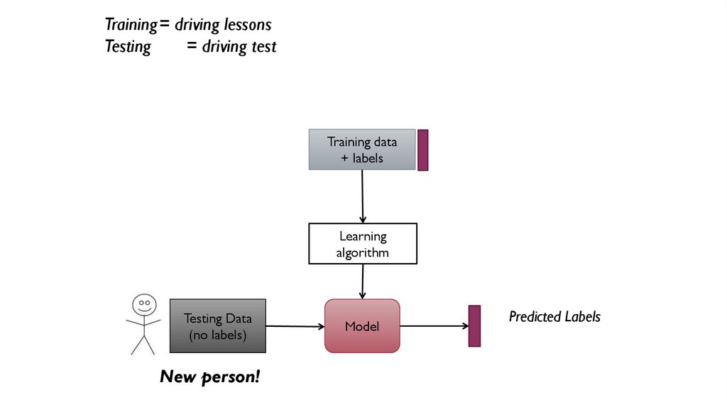
Training= driving lessonsTesting
= driving test
Training data
+ labels
Learning
algorithm
Testing Data
(no labels)
New person!
Model
Predicted Labels
83.
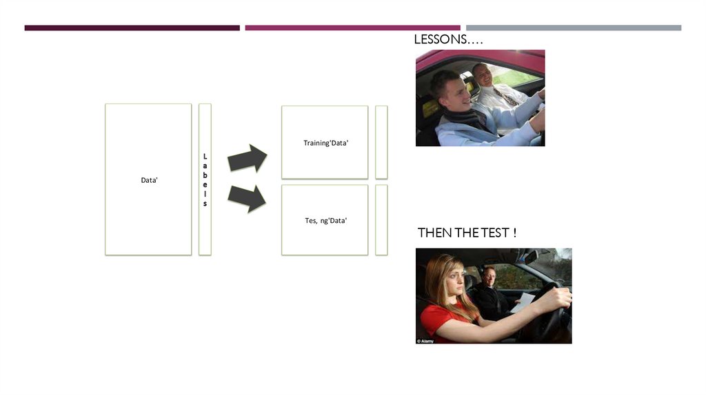
LESSONS….2.1. BUILDING & EVALUAT ING A ‘MODEL’ OF T HE DATA
13
Training'Data'
Data'
Tes, ng'Data'
THEN THE TEST !
Figure 2.6: Splitting data into training and testing sets.
If we were t o just learn t he model (t rain) on t he ent ire dat aset , we might
just learn t he charact erist ics of t his dat aset , e↵ect ively ne-tuning our model so
it would just work well here, as opposed t o working well out in t he real world as
well. T his ne-tuning is known in t echnical t erms as over tting, and is obviously OV ERFI T T I NG
somet hing we wish t o avoid.
84.
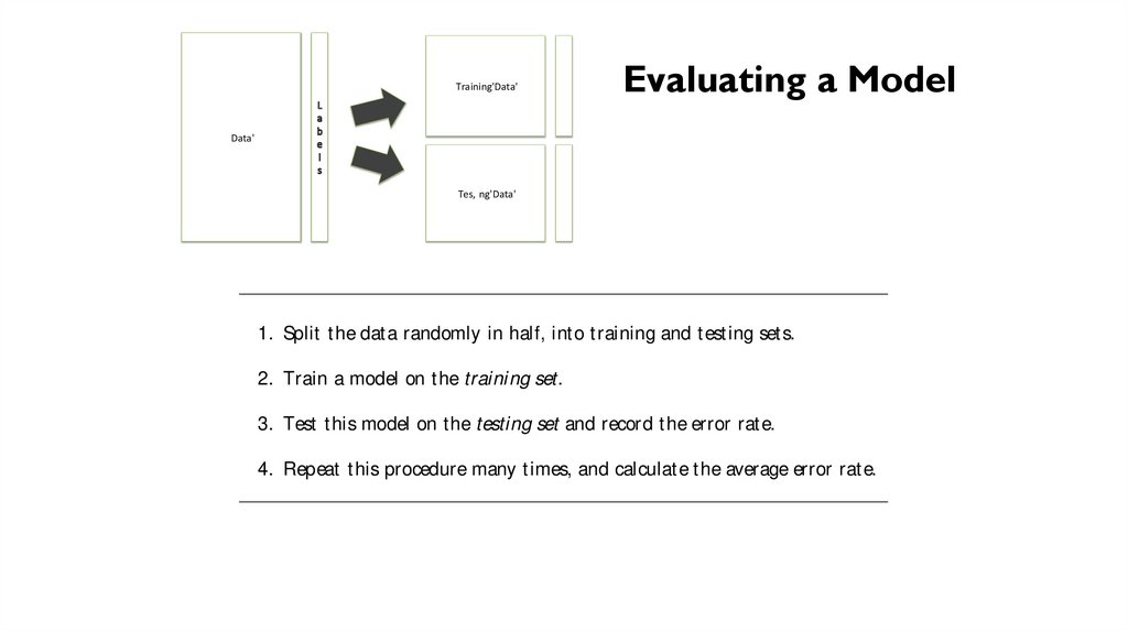
Figure 2.6: Splitting data into training and testing sets.Evaluating
a
Model
If we were t o just learn t he model (t rain) on t he ent ire dat aset , we might
Training'Data'
just learn t he charact erist ics of t his dat aset , e↵ect ively ne-tuning our model so
it would just work well here, as opposed t o working well out in t he real world as
well. T his ne-tuning is known in t echnical t erms as over tting, and is obviously OV ERFI T T ING
Tes, ng'Data'
somet hing we wish t o avoid.
Data'
Wit h t his in mind, we can present pseudo-code for a good learning prot ocol:
Figure 2.6: Splitting data into training and testing sets.
If we were t o just learn t he model (t rain) on t he ent ire dat aset , we might
1. Split t he dat a randomly in half, int o t raining and t est ing set s.
just learn t he charact erist ics of t his dat aset , e↵ect ively ne-tuning our model so
it would just work well here, as opposed t o working well out in t he real world as
Train
model ton
t he
set.
well. T his ne-tuning is2.
known
in a
t echnical
erms
astraining
over tting,
and is obviously OV ERFI T T I NG
somet hing we wish t o avoid.
3. Test t his model on t he testing set and record t he error rat e.
Wit h t his in mind, we can present pseudo-code for a good learning prot ocol:
4. Repeat t his procedure many t imes, and calculat e t he average error rat e.
1. Split t he dat a randomly in half, int o t raining and t est ing set s.
Nottraining
ice t hatset.we repeat ed t his many t imes, split t ing t he dat a randomly. On
2. Train a model on t he
each split , t he model was t rained, and t he t est set it was evaluat ed on was
3. Test t his modelkind
on t he
and record
rat e. ‘score’ t hat we assign t o t he model is
of testing
like aset
‘mock’
exam.t heTerror
he nal
85.
The Nearest NeighbourClassifier
86.
The Nearest Neighbour Ruleheight
Person
Weight
Height
1
2
3
4
5
…
16
17
18
19
20
…
63kg
55kg
75kg
50kg
57kg
…
85kg
93kg
75kg
99kg
100kg
…
190cm
185cm
202cm
180cm
174cm
150cm
145cm
130cm
163cm
171cm
“TRAINING” DATA
weight
“TESTING” DATA
Who’s this guy?
- player or dancer?
height = 180cm
weight = 78kg
87.
The Nearest Neighbour Ruleheight
Person
Weight
Height
1
2
3
4
5
…
16
17
18
19
20
…
63kg
55kg
75kg
50kg
57kg
…
85kg
93kg
75kg
99kg
100kg
…
190cm
185cm
202cm
180cm
174cm
150cm
145cm
130cm
163cm
171cm
“TRAINING” DATA
weight
height = 180cm
weight = 78kg
1. Find nearest neighbour
2. Assign the same class
88.
Supervised Learning Pipeline for Nearest NeighbourTraining data
Learning algorithm
(do nothing)
Testing Data
(no labels)
Model
(memorize the
training data)
Predicted Labels
89.
The K-Nearest Neighbour ClassifierTesting point x
For each training datapoint x’
measure distance(x,x’)
End
Sort distances
Select K nearest
Assign most common class
Person
Weight
Height
1
2
3
4
5
…
16
17
18
19
20
…
63kg
55kg
75kg
50kg
57kg
…
85kg
93kg
75kg
99kg
100kg
…
190cm
185cm
202cm
180cm
174cm
150cm
145cm
130cm
163cm
171cm
“TRAINING” DATA
height
weight
90.
Quick reminder: Pythagoras’ theorem. . .
measure distance(x,x’)
. . .
a
c
a 2 b2 c 2
b
So....
a.k.a. “Euclidean” distance
c a 2 b2
height
distance ( x, x' )
( xi x 'i ) 2
i
weight
91.
The K-Nearest Neighbour ClassifierTesting point x
For each training datapoint x’
measure distance(x,x’)
End
Sort distances
Select K nearest
Assign most common class
Person
Weight
Height
1
2
3
4
5
…
16
17
18
19
20
…
63kg
55kg
75kg
50kg
57kg
…
85kg
93kg
75kg
99kg
100kg
…
190cm
185cm
202cm
180cm
174cm
150cm
145cm
130cm
163cm
171cm
“TRAINING” DATA
height
Seems sensible.
But what are the disadvantages?
weight
92.
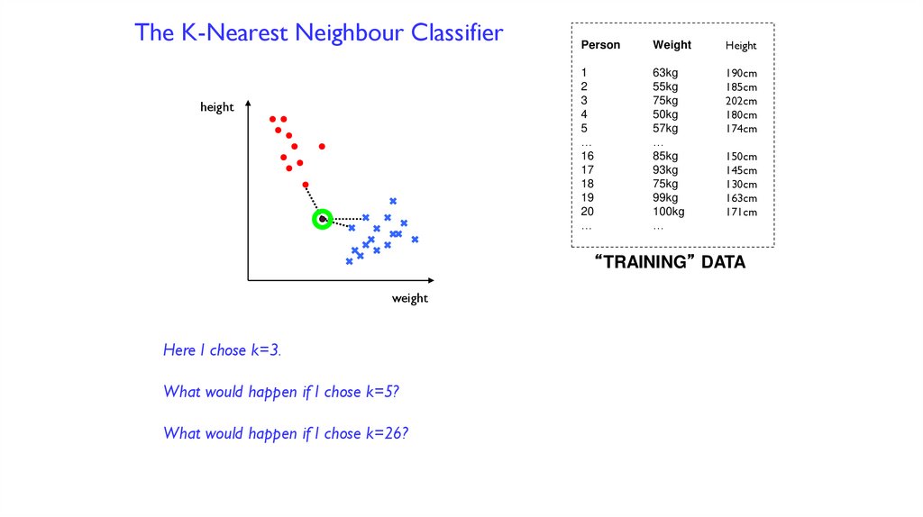
The K-Nearest Neighbour Classifierheight
Person
Weight
Height
1
2
3
4
5
…
16
17
18
19
20
…
63kg
55kg
75kg
50kg
57kg
…
85kg
93kg
75kg
99kg
100kg
…
190cm
185cm
202cm
180cm
174cm
150cm
145cm
130cm
163cm
171cm
“TRAINING” DATA
weight
Here I chose k=3.
What would happen if I chose k=5?
What would happen if I chose k=26?
93.
The K-Nearest Neighbour Classifierheight
Person
Weight
Height
1
2
3
4
5
…
16
17
18
19
20
…
63kg
55kg
75kg
50kg
57kg
…
85kg
93kg
75kg
99kg
100kg
…
190cm
185cm
202cm
180cm
174cm
150cm
145cm
130cm
163cm
171cm
“TRAINING” DATA
weight
Any point on the left of this “boundary” is closer to the red circles.
Any point on the right of this “boundary” is closer to the blue crosses.
This is called the “decision boundary”.
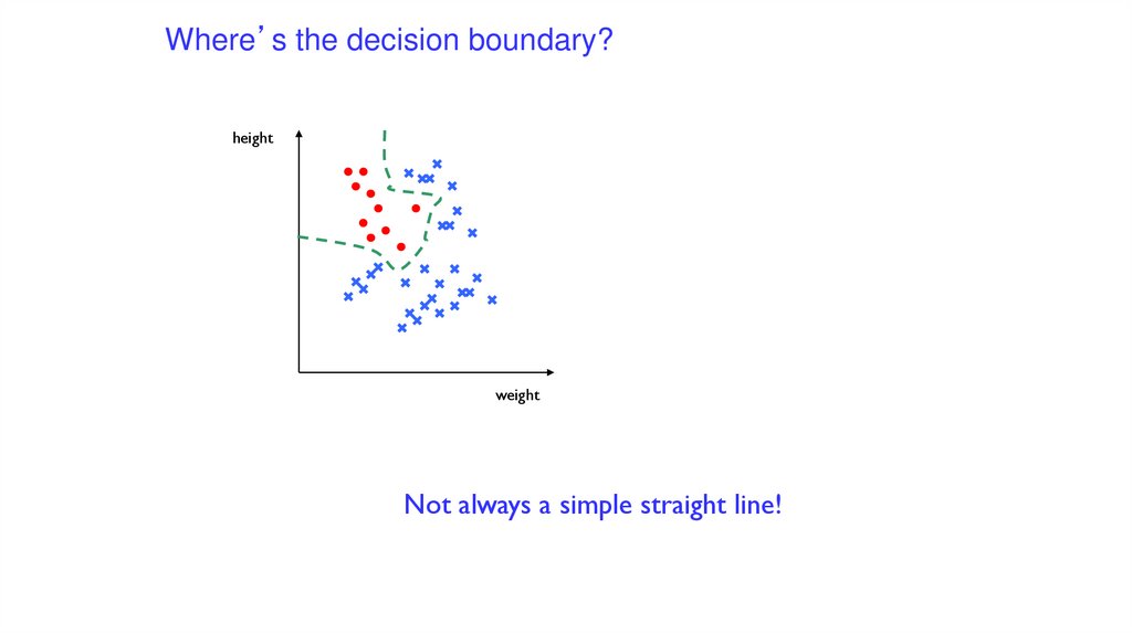
94.
Where’s the decision boundary?height
weight
Not always a simple straight line!
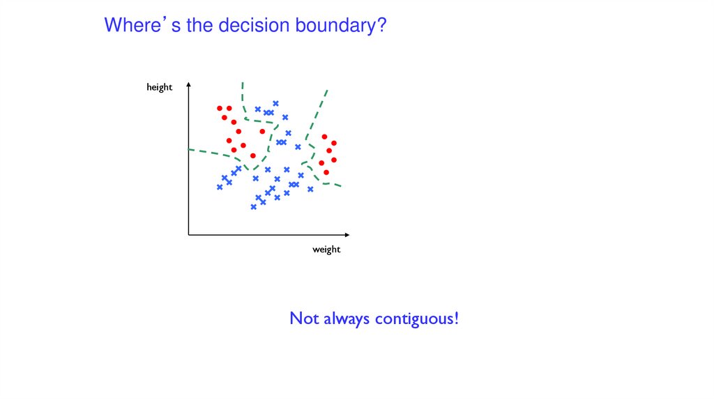
95.
Where’s the decision boundary?height
weight
Not always contiguous!
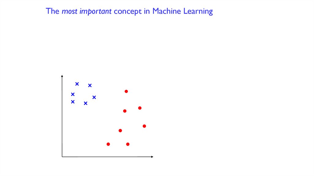
96.
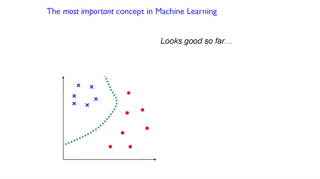
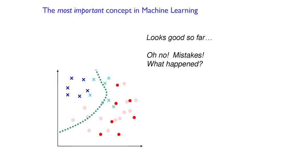
The most important concept in Machine Learning97.
The most important concept in Machine LearningLooks good so far…
98.
The most important concept in Machine LearningLooks good so far…
Oh no! Mistakes!
What happened?
99.
The most important concept in Machine LearningLooks good so far…
Oh no! Mistakes!
What happened?
We didn’t have all the data.
We can never assume that we do.
This is called “OVER-FITTING”
to the small dataset.
100.
Pretty dumb! Where’s the learning!Training data
Learning algorithm
(do nothing)
Testing Data
(no labels)
Model
(memorize the
training data)
Predicted Labels
101.
Now, how is this problem likehandwriting recognition?
height
weight
102.
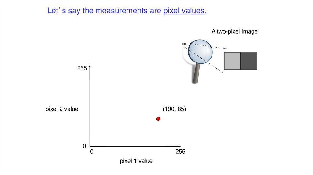
Let’s say the measurements are pixel values.A two-pixel image
255
pixel 2 value
(190, 85)
0
0
255
pixel 1 value
103.
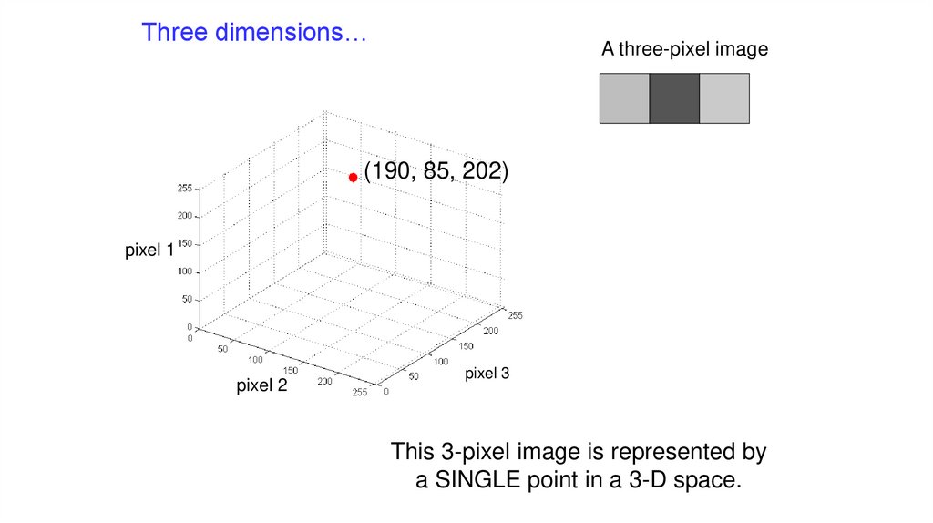
Three dimensions…A three-pixel image
(190, 85, 202)
pixel 1
pixel 2
pixel 3
This 3-pixel image is represented by
a SINGLE point in a 3-D space.
104.
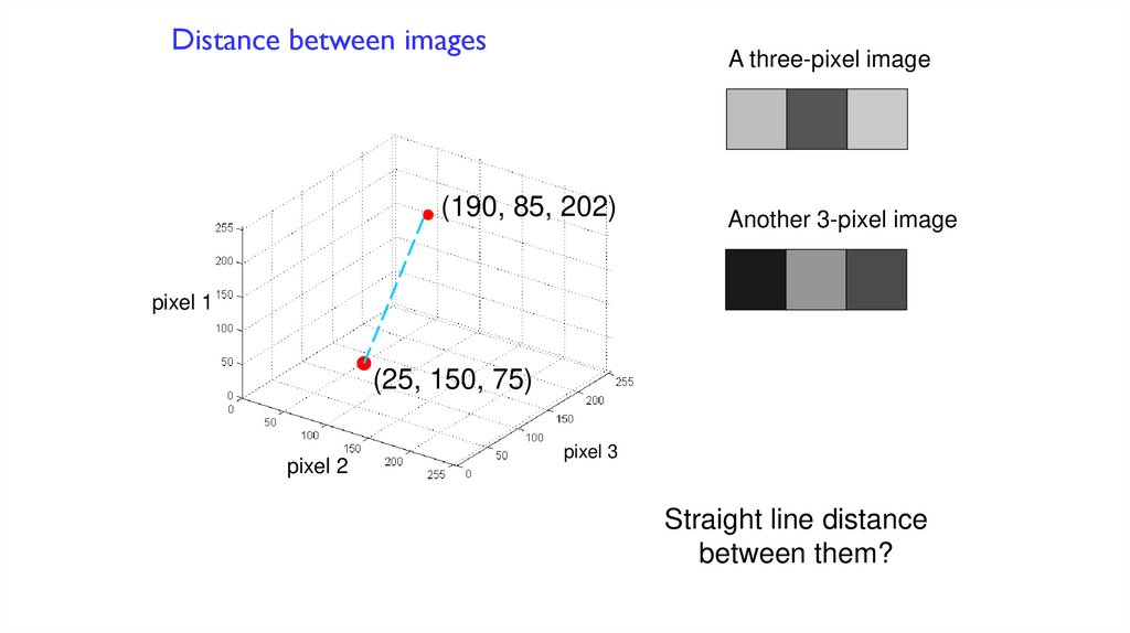
Distance between imagesA three-pixel image
(190, 85, 202)
Another 3-pixel image
pixel 1
(25, 150, 75)
pixel 2
pixel 3
Straight line distance
between them?
105.
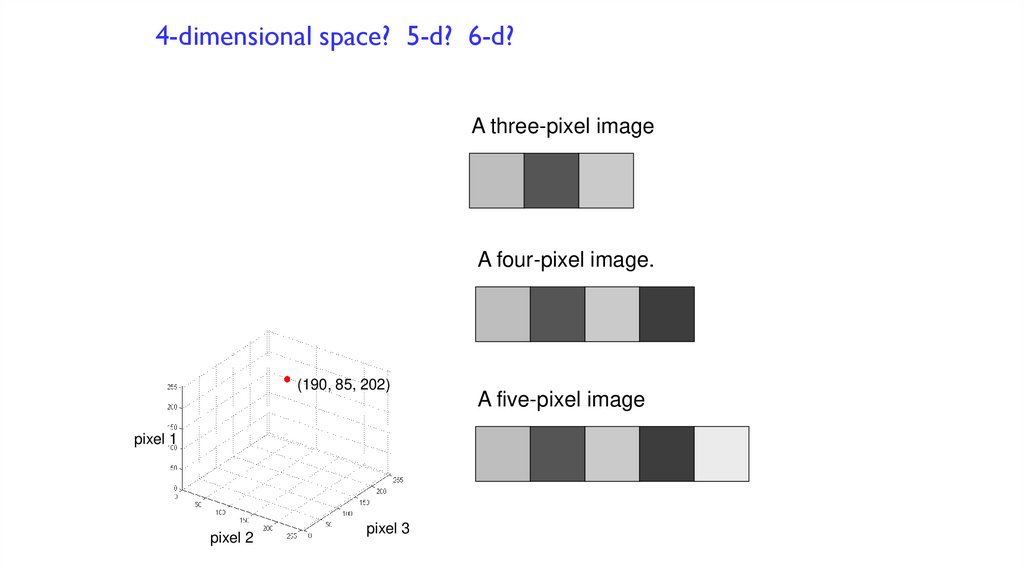
4-dimensional space? 5-d? 6-d?A three-pixel image
A four-pixel image.
(190, 85, 202)
pixel 1
pixel 2
pixel 3
A five-pixel image
106.
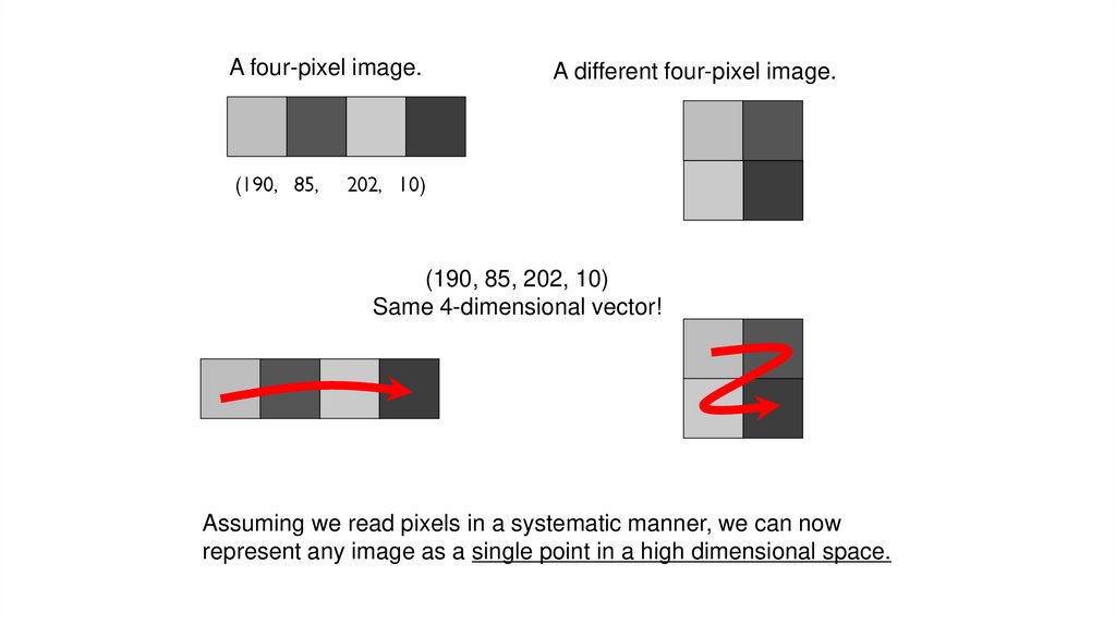
A four-pixel image.(190, 85,
A different four-pixel image.
202, 10)
(190, 85, 202, 10)
Same 4-dimensional vector!
Assuming we read pixels in a systematic manner, we can now
represent any image as a single point in a high dimensional space.
107.
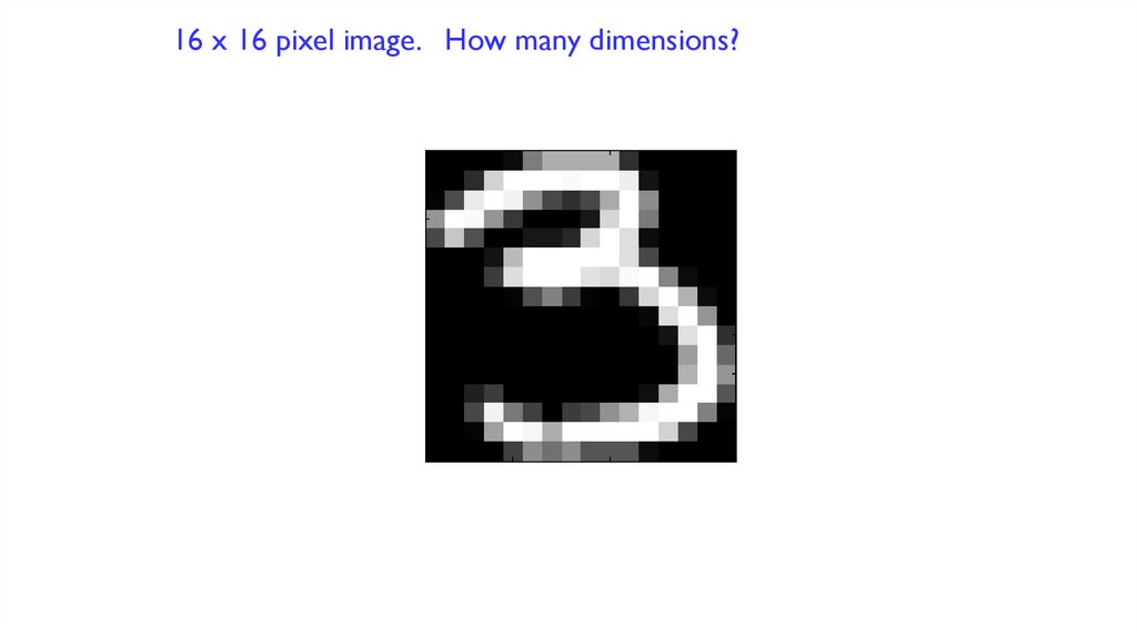
16 x 16 pixel image. How many dimensions?108.
We can measure distance in 256 dimensional space.distance ( x, x' )
?
i 256
( x x' )
i 1
i
i
2
109.
Which is the nearest neighbour to our ‘3’ ?maybe
maybe
probably
not