Basis Sets and Pseudopotentials

1. Basis Sets and Pseudopotentials

2. Slater-Type Orbitals (STO’s)

f
STO
abc
a b c -zr
(x,y,z) = Nx y z e
• N is a normalization constant
• a, b, and c determine the angular momentum, i.e.
L=a+b+c
• ζ is the orbital exponent. It determines the size of the
orbital.
• STO exhibits the correct short- and long-range behavior.
• Resembles H-like orbitals for 1s
• Difficult to integrate for polyatomics

3. Gaussian-Type Orbitals (GTO’s)

f
GTO
abc
b c -zr 2
(x,y,z) = Nx y z e
a
• N is a normalization constant
• a, b, and c determine the angular momentum, i.e.
L=a+b+c
• ζ is the orbital exponent. It determines the size of the
orbital.
• Smooth curve near r=0 instead of a cusp.
• Tail drops off faster a than Slater orbital.
• Easy to integrate.

4. Contracted Basis Sets

c(CGTO) = å ai ci (PGTO)
b
i=a
• P=primitive, C=contracted
• Reduces the number of basis functions
• The contraction coefficients, αi, are constant
• Can be a segmented contraction or a general contraction

5. Contracted Basis Sets

Segmented Contraction
CGTO-1
CGTO-2
PGTO-1
PGTO-2
PGTO-3
PGTO-4
PGTO-5
PGTO-6
PGTO-7
PGTO-8
PGTO-9
PGTO-10
Jensen, Figure 5.3, p. 202
General Contraction
CGTO-3
CGTO-1
CGTO-2
CGTO-3

6.

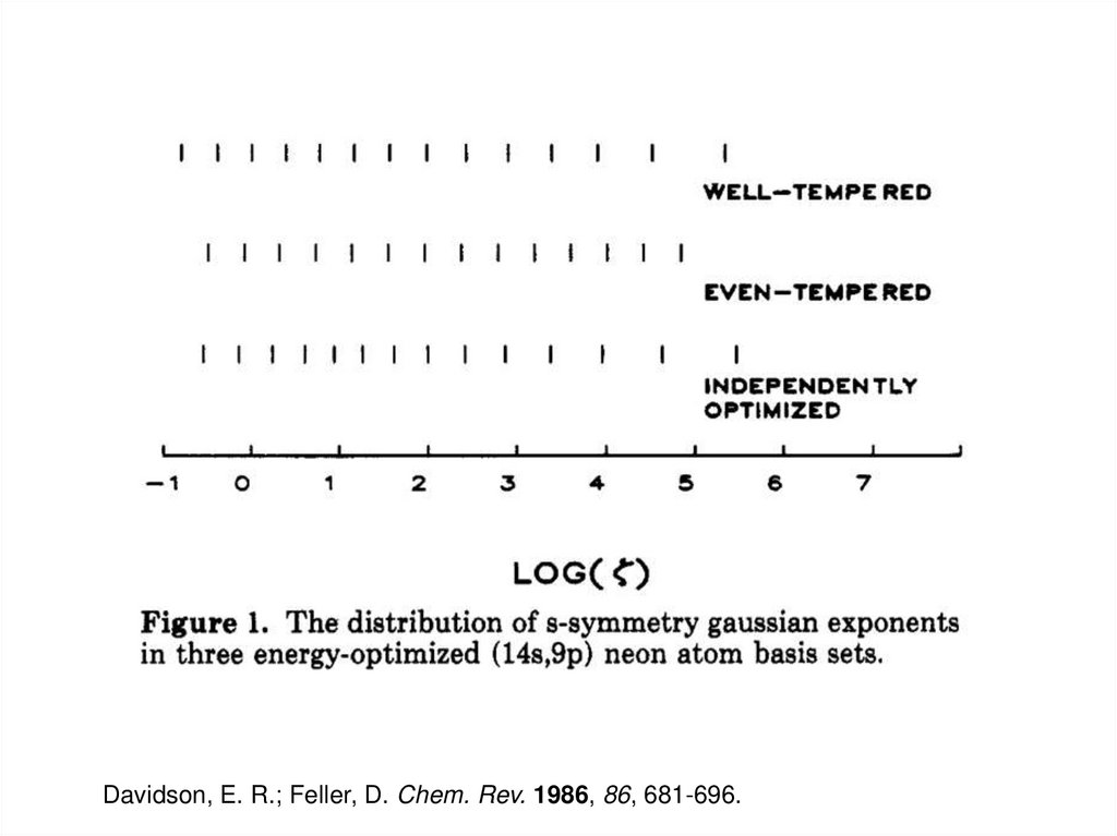
STO-NG: STO approximated by linear combination of N Gaussians

7. Even-tempered Basis Sets

b c -zr 2
f abc (x,y,z) = Nx y z e
a
z i = abi
• Same functional form as the Gaussian functions used earlier
• The exponent, ζ, is fitted to two parameters with different
α and β for s, p, d, etc. functions.
• Successive exponents are related by a geometric series
- log(ζ) are evenly spaced
Reudenberg, K., et Al., Energy, Structure and Reactivity, Proceedings of the 1972
Boulder Conference; Wiley: New York, 1973.
Reeves, C. M. J. Chem Phys. 1963, 39, 1.

8. Well-tempered Basis Sets

b c -zr 2
f abc (x,y,z) = Nx y z e
a
k -1
k d
K
z i = ab [1+ g( ) ],
k = 1,2,...,K
• α, β, γ, and δ are parameters optimized to minimize the SCF
energy
• Exponents are shared for s, p, d, etc. functions
Huzinaga, S. et Al., Can. J. Chem. 1985, 63, 1812.

9.

Davidson, E. R.; Feller, D. Chem. Rev. 1986, 86, 681-696.

10. Plane Wave Basis Sets

• Used to model infinite systems (e.g. metals, crystals, etc.)
• In infinite systems, molecular orbitals become bands
• Electrons in bands can be described by a basis set of plane
waves of the form
ck (r) = e
ik×r
• The wave vector k in a plane wave function is similar to the
orbital exponent in a Gaussian function
• Basis set size is related to the size of the unit cell rather than
the number of atoms

11. Polarization Functions

Similar exponent as valence function
Higher angular momentum (l+1)
Uncontracted Gaussian (coefficient=1)
Introduces flexibility in the wave function
by making it directional
• Important for modeling chemical bonds

12. Diffuse Functions

• Smaller exponent than valence functions
(larger spatial extent)
• Same angular momentum as valence
functions
• Uncontracted Gaussian (coefficient=1)
• Useful for modeling anions, excited states and
weak (e.g., van der Waals) interactions

13. Cartesian vs. Spherical

Cartesians:
s – 1 function
p – 3 functions
d – 6 functions
f – 10 functions
Sphericals:
s – 1 function
p – 3 functions
d – 5 functions
f – 7 functions
Look at the d functions:
In chemistry, there should be 5 d functions (usually chosen to be
,d 2 2
x -y
d z2, d xy, d,xzand d. yz These are “pure angular momentum” functions.
But it is easier to write a program to use Cartesian functions (
d xy, d xz, and d. yz
, d,x 2 d, y 2 d z 2

14. Cartesian vs. Spherical

Suppose we calculated the energy of HCl using a
cc-pVDZ basis set using Cartesians then again
using sphericals.
Which calculation produces the lower energy?
Why?

15. Pople Basis Sets

• Optimized using Hartree-Fock
• Names have the form
k-nlm++G** or k-nlmG(…)
• k is the number of contracted Gaussians used for core
orbitals
• nl indicate a split valence
• nlm indicate a triple split valence
• + indicates diffuse functions on heavy atoms
• ++ indicates diffuse functions on heavy atoms and hydrogens

16. Pople Basis Sets

Examples:
6-31G
Three contracted Gaussians for the core with the valence
represented by three contracted Gaussians and one
primitive Gaussian
6-31G* Same basis set with a polarizing function added
6-31G(d) Same as 6-31G*
6-31G** Polarizing functions added to hydrogen and heavy atoms
6-31G(d,p) Same as 6-31G**
6-31++G 6-31G basis set with diffuse functions on hydrogen and
heavy atoms
The ** notation is confusing and not used for larger basis sets:
6-311++G(3df, 2pd)

17. Dunning Correlatoin Consistent Basis Sets

• Optimized using a correlated method (CIS, CISD, etc.)
• Names have the form
aug-cc-pVnZ-dk
• “aug” denotes diffuse functions (optional)
• “cc” means “correlation consistent”
• “p” indicates polarization functions
• “VnZ” means “valence n zeta” where n is the number of
functions used to describe a valence orbital
• “dk” indicates that the basis set was optimized for relativistic
calculations
• Very useful for correlated calculations, poor for HF
• Size of basis increases rapidly with n

18. Dunning Basis Sets

Examples:
cc-pVDZ
Double zeta with polarization
aug-cc-pVTZ
Triple zeta with polarization and
diffuse functions
cc-pV5Z-dk
Quintuple zeta with polarization optimized for
relativistic effects

19. Extrapolate to complete basis set limit

Most useful for electron correlation methods
P(lmax) = P(CBS) + A( lmax)-3
P(n) = P(CBS) + A( n)-3
n refers to cc basis set level: for for DZ, 3 for TZ, etc.
Best to use TZP and better
http://molecularmodelingbasics.blogspot.dk/2012/06/comp
lete-basis-set-limit-extrapolation.html
TCA, 99, 265 (1998)

20. Basis Set Superposition Error

• Occurs when a basis function centered at one nucleus
contributes the the electron density around another nucleus
• Artificially lowers the total energy
• Frequently occurs when using an unnecessarily large basis set
(e.g. diffuse functions for a cation)
• Can be corrected for using the counterpoise correction.
- Counterpoise usually overcorrects
- Better to use a larger basis set

21. Counterpoise Correction

DE CP = E(A)ab + E(B)ab - E(A)a - E(B)b
• E(A)ab is the energy of fragment A with the basis functions for
A+B
• E(A)a is the energy of fragment A with the basis functions
centered on fragment A
• E(B)ab and E(B)b are similarly defined

22. Additional Information

EMSL Basis Set Exchange:
https://bse.pnl.gov/bse/portal
Further reading:
Davidson, E. R.; Feller, D. Chem. Rev. 1986, 86, 681-696.
Jensen, F. “Introduction to Computational Chemistry”, 2nd
ed., Wiley, 2009, Chapter 5.

23. Effective Core Potentials (ECPs) and Model Core Potentials (MCPs)

24. Frozen Core Approximation

All electron Fock operator:
Nuclei
å
F = hkinetic -
A
occ
ZA
+ å (J j - K j )
rA
j
Partition the core (atomic) orbitals and the valence orbitals:
Nuclei
F = hkinetic -
å
Z
valence
ZA Nuclei core A
+ å å (Jc - K cA ) + å (Jv - K v )
rA
A
c
v
):Z*
Introduce a modified nuclear charge (
Nuclei
F =h
kinetic
-
å
A
ZA*
+
rA
valence
å
v
A
Nuclei
(Jv - K v ) +
å
A
= ZA - Zcore
å Z core core å Nuclei core
å- A + å JcA å- å å K cA
å rA
å A c
c
VCoulomb
Approximation made: atomic core orbitals are not allowed to
change upon molecular formation; all other orbitals stay
orthogonal to these AOs
VExchange

25. Pseudopotentials - ECPs

Effective core potentials (ECPs) are pseudopotentials that
replace core electrons by a potential fit to all-electron
calculations. Scalar relativisitc effects (e.g. mass-velocity
and Darwin) are included via a fit to relativistic orbitals.
Two schools of though:
1. Shape consistent ECPs
(e.g. LANLDZ RECP, etc.)
2. Energy consistent ECPs
(e.g. Stüttgart LC/SC RECP, etc.)

26. Shape Consistent ECPs

• Nodeless pseudo-orbitals that resemble the valence orbitals in the
bonding region
³y v ( r ) (r ³ rc )
y v ( r ) ®y˜ v ( r ) = ³
³ f v (r ) (r < rc )
Original orbital in the outer region
Smooth polynomial expansion in the
inner region
• The fit is usually done to either the large component of the Dirac wave
function or to a 3rd order Douglas-Kroll wave function
• Creating a normalized shape consistent orbital requires mixing in
virtual orbitals
• Usually gives accurate bond lengths and structures

27. Energy Consistent ECPs

• Approach that tries to reproduce the low-energy atomic spectrum
(via correlated calculations)
åLow-lying
å
levels
2
å
PP
Re ference å
minå å wI ( EI - EI
)
å
å I
å
å
å
• Usually fit to 3rd order Douglas-Kroll
• Difference in correlation energy due to the nodeless valence orbitals is
included in the fit
• Small cores are still sometimes necessary to obtain reliable results
(e.g. actinides)
• Cheap core description allows for a good valence basis set (e.g. TZVP)
• Provides accurate results for many elements and bonding situations

28. Pseudo-orbitals

Visscher, L., “Relativisitic Electronic Structure Theory”, 2006 Winter School, Helkinki, Finland.

29. Large and Small Core ECPs

Jensen, Figure 5.7, p. 224.

30. Pseudopotentials - MCPs

• Model Core Potentials (MCP) provide a
computationally feasible treatment of heavy elements.
• MCPs can be made to include scalar relativistic effects
- Mass-velocity terms
- Darwin terms
• Spin orbit effects are neglected.
- Inclusion of spin-orbit as a perturbation has been
proposed
• MCPs for elements up to and including the lanthanides
are as computationally demanding as large core ECPs.

31. MCP Formulation

All-electron (AE) Hamiltonian:
N
Natom
N
1
ZL ZM
AE
ˆ
H (1,2, ,N) = å hi + å + å
r L>M RLM
i=1
i> j ij
MCP Hamiltonian:
(
)
Nv
Nv
Natom
i=1
i> j
L>M
1
MCP
ˆ
H 1,2, ,N = å hi + å +
v
rij
å
( ZL - NL,Core )( ZM - NM ,Core)
RLM
• First term is the 1 electron MCP Hamiltonian
• Second term is electron-electron repulsion (valence only)
• Third term is an effective nuclear repulsion
Huzinaga, S.; Klobukowski, M.; Sakai, Y. J. Phys. Chem. 1982, 88, 21.
Mori, H; Eisaku, M Group Meeting, Nov. 8, 2006.

32. 1-electron Hamiltonian

All-electron (AE) Hamiltonian:
N
Natom
N
1
ZL ZM
AE
ˆ
H (1,2, ,N) = å hi + å + å
r L>M RLM
i=1
i> j ij
MCP Hamiltonian:
atom
ZL - NL,Core )( ZM - NM ,Core )
1
(
MCP
ˆ
H 1,2, ,N = å hi + å + å
v
r L>M
RLM
i=1
i> j ij
(
)
Nv
Nv
N
• First term is the 1 electron MCP Hamiltonian
• Second term is electron-electron repulsion (valence only)
• Third term is an effective nuclear repulsion
Huzinaga, S.; Klobukowski, M.; Sakai, Y. J. Phys. Chem. 1982, 88, 21.
Mori, H; Eisaku, M Group Meeting, Nov. 8, 2006.

33. MCP Nuclear Attraction

3
3
³
³
Z
N
MCP
2
2
K
K ,core
VK (r i ) = ³1+ ³ AI exp( -a I riK ) + ³ BJ riK exp( -bJ riK ) ³
riK
³ I
³
J
• AI, αI, BJ, and βJ are fitted MCP parameters
• MCP parameters are fitted to 3rd order Douglas-Kroll orbitals
Huzinaga, S.; Klobukowski, M.; Sakai, Y. J. Phys. Chem. 1982, 88, 21.
Mori, H; Eisaku, M Group Meeting, Nov. 8, 2006.

34. MCP vs. ECP

■ 6s Orbital of Au atom
QRHF
ECP
MCP
rR(r) / a.u.
0.8
• ECPs “smooth out” the core,
eliminating the radial nodal
structure
0.4
• MCPs retain the correct radial
nodal structure
0.0
-0.4
0
2
4
r / a.u.
6
8
10
Mori, H; Eisaku, M Group Meeting, Nov. 8, 2006.