ASB1114: Regression

1.

ASB1114:
Regression

2.

The two-variable linear regression model
Estimation
The population (‘true’) regression line:
The linear regression model is used to investigate casual relationships between 2 [or more]
random variables.
For example, let xi = disposable income of household i in 2013
yi = consumer expenditure of household i in 2013
We expect to find positive relationship between xi and yi. We might also expect that xi
(disposable income) largely determines yi (consumer expenditure).

3.

The two-variable linear regression model
Estimation
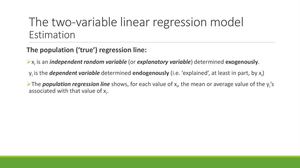
The population (‘true’) regression line:
xi is an independent random variable (or explanatory variable) determined exogenously.
yi is the dependent variable determined endogenously (i.e. ‘explained’, at least in part, by xi)
The population regression line shows, for each value of xi, the mean or average value of the yi’s
associated with that value of xi.

4.

The two-variable linear regression model
Estimation
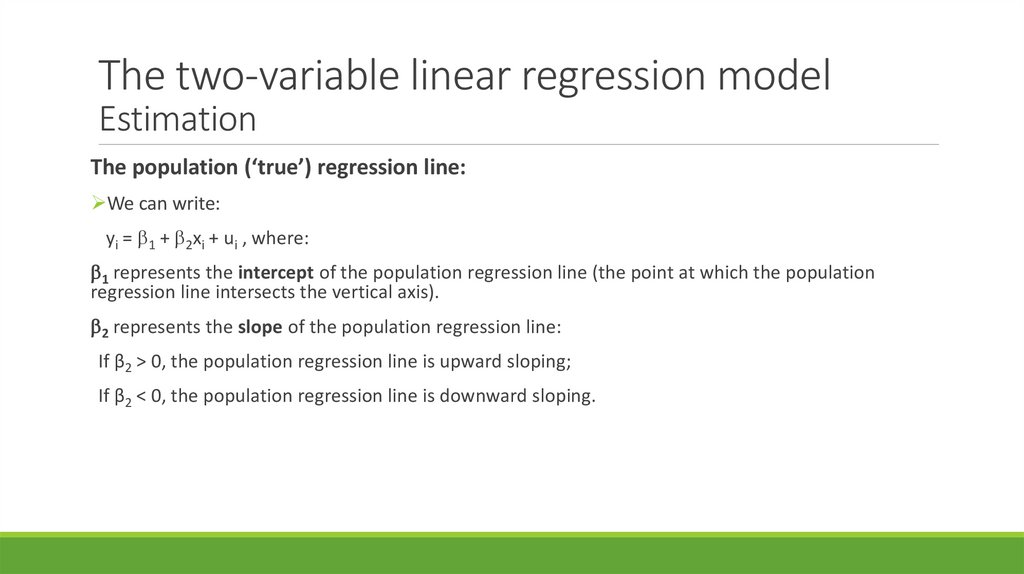
The population (‘true’) regression line:
We can write:
yi = 1 + 2xi + ui , where:
1 represents the intercept of the population regression line (the point at which the population
regression line intersects the vertical axis).
2 represents the slope of the population regression line:
If β2 > 0, the population regression line is upward sloping;
If β2 < 0, the population regression line is downward sloping.

5.

The two-variable linear regression model
Estimation
The population (‘true’) regression line:
We can write:
yi = 1 + 2xi + ui , where:
ui is the error term. In practice, the relationship between xi and yi for any particular household is
never described exactly by the position of the population regression line. Each individual
household is located somewhere either above or below the line (their expenditure is either a bit
more or bit less than the average for households of their income level). The error term allows for
this divergence.
We assume E(ui)=0 and var(ui) = 2.

6.

The two-variable linear regression model
Estimation
The population (‘true’) regression line:
The population scatter diagram plots the values of xi and yi against one another for all
households in the population.
A regression analysis describes the relationship between xi and yi that is summarised by this
diagram.
ui is represented diagrammatically by the vertical distance between the ‘point’ for the i’th
household, and the population regression line.

7.

Population scatter diagram
yi
slope = 2
E(Yi|xi)= 1+ 2xi
1
xi

8.

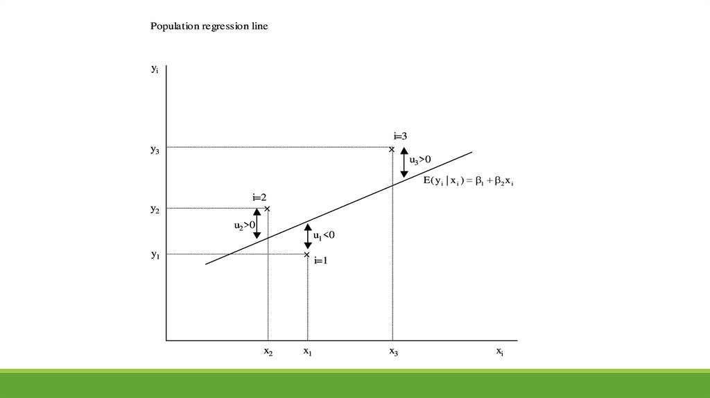
Population regression line
yi
i=3
y3
u3 >0
E ( y i | x i ) 1 2 x i
y2
i=2
u2 >0
u1 <0
y1
x2
x1
i=1
x3
xi

9.

The two-variable linear regression model
Estimation
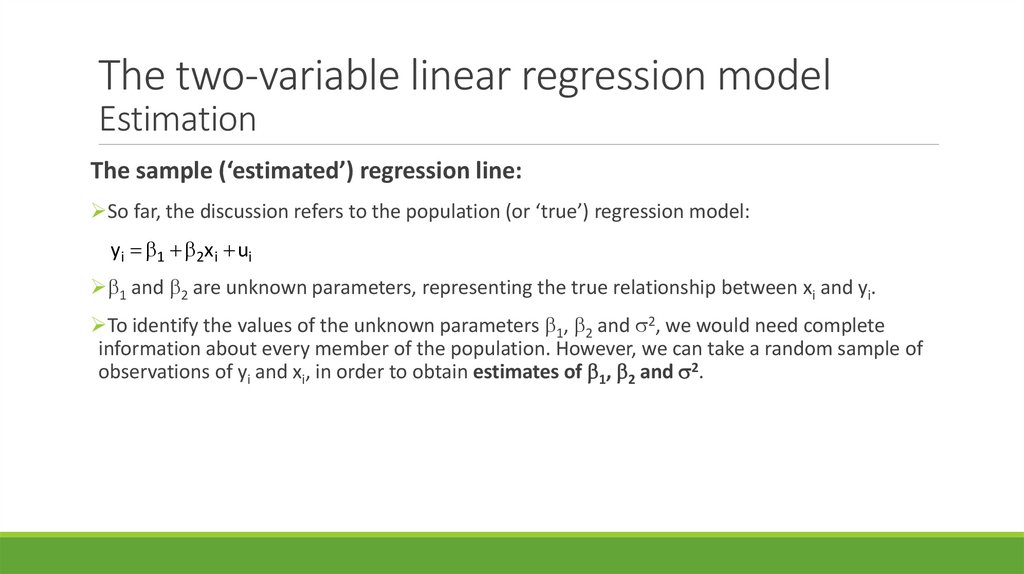
The sample (‘estimated’) regression line:
So far, the discussion refers to the population (or ‘true’) regression model:
y i 1 2x i ui
1 and 2 are unknown parameters, representing the true relationship between xi and yi.
To identify the values of the unknown parameters 1, 2 and 2, we would need complete
information about every member of the population. However, we can take a random sample of
observations of yi and xi, in order to obtain estimates of 1, 2 and 2.

10.

The two-variable linear regression model
Estimation
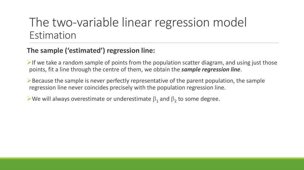
The sample (‘estimated’) regression line:
If we take a random sample of points from the population scatter diagram, and using just those
points, fit a line through the centre of them, we obtain the sample regression line.
Because the sample is never perfectly representative of the parent population, the sample
regression line never coincides precisely with the population regression line.
We will always overestimate or underestimate 1 and 2 to some degree.

11.

The two-variable linear regression model
Estimation
The sample (‘estimated’) regression line:
Therefore it is important to develop notation to distinguish the ‘true’ parameters ( 1 and 2)
from their sample estimates, as follows:
Population (‘true’) model: y i 1 2x i ui (for i=1....N where N=population size)
Sample (‘estimated’) model: y i ˆ 1 ˆ 2x i ei (for i=1.....n where n=sample size)

12.

The two-variable linear regression model
Estimation
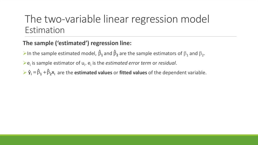
The sample (‘estimated’) regression line:
In the sample estimated model, ̂1 and ̂2 are the sample estimators of 1 and 2.
ei is sample estimator of ui. ei is the estimated error term or residual.
ŷ i ˆ 1 ˆ 2x i are the estimated values or fitted values of the dependent variable.

13.

The two-variable linear regression model
Estimation
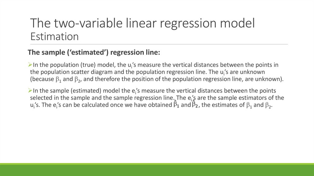
The sample (‘estimated’) regression line:
In the population (true) model, the ui’s measure the vertical distances between the points in
the population scatter diagram and the population regression line. The ui’s are unknown
(because 1 and 2, and therefore the position of the population regression line, are unknown).
In the sample (estimated) model the ei’s measure the vertical distances between the points
selected in the sample and the sample regression line. The ei’s are the sample estimators of the
ui’s. The ei’s can be calculated once we have obtained ̂1 and ̂2 , the estimates of 1 and 2.

14.

Sample scatter diagram
yi
slope = ̂ 2
ŷ i ˆ 1 ˆ 2 x i
E(Yi|xi)= 1+ 2xi
̂1
xi

15.

Population and sample regression lines
yi
i=3
y3
e3 >0
y2
i=2
e >0
E ( y i | x i ) 1 2 x i
ŷ i ˆ 1 ˆ 2 x i
2
e1 <0
y1
x2
x1
i=1
x3
xi

16.

Ordinary Least Squares estimation of 1
and 2
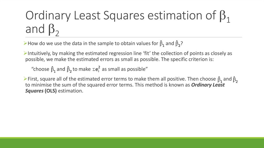
How do we use the data in the sample to obtain values for ̂1 and ̂2?
Intuitively, by making the estimated regression line ‘fit’ the collection of points as closely as
possible, we make the estimated errors as small as possible. The specific criterion is:
“choose ̂1 and ̂2 to make e2i as small as possible”
First, square all of the estimated error terms to make them all positive. Then choose ̂1 and ̂2
to minimise the sum of the squared error terms. This method is known as Ordinary Least
Squares (OLS) estimation.

17.

Ordinary Least Squares estimation of 1
and 2
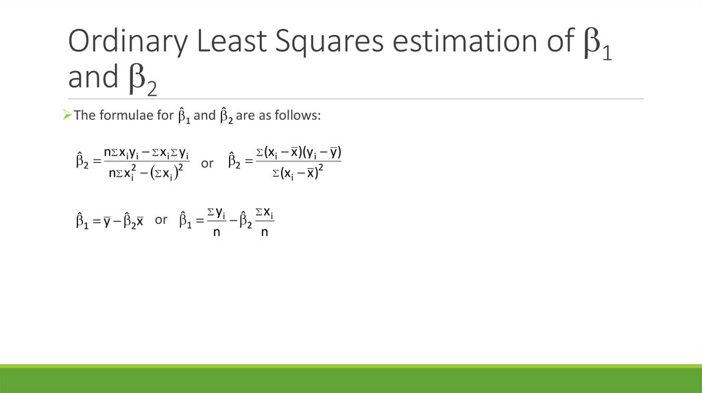
The formulae for ̂1 and ̂2 are as follows:
(x x )(y y)
n x iy i x i y i
i
i
ˆ
ˆ 2
or
2
2
(x x )
n x 2i x i 2
i
ˆ 1 y ˆ 2 x or ˆ 1 y i ˆ 2 x i
n
n

18.

Ordinary Least Squares estimation of 1
and 2
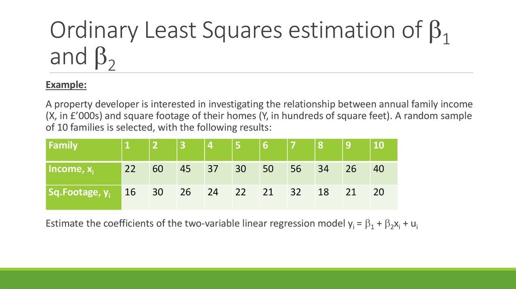
Example:
A property developer is interested in investigating the relationship between annual family income
(X, in £’000s) and square footage of their homes (Y, in hundreds of square feet). A random sample
of 10 families is selected, with the following results:
Family
1
2
3
4
5
6
7
8
9
10
Income, xi
22
60
45
37
30
50
56
34
26
40
Sq.Footage, yi
16
30
26
24
22
21
32
18
21
20
Estimate the coefficients of the two-variable linear regression model yi = 1 + 2xi + ui

19.

Ordinary Least Squares estimation of 1
and 2
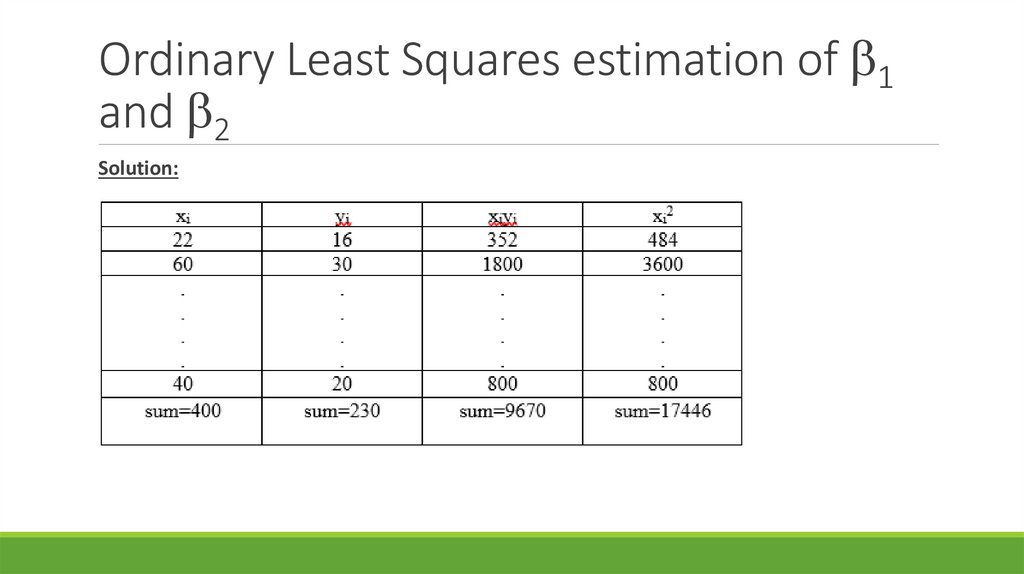
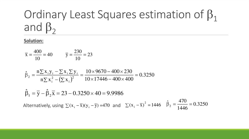
Solution:

20.

Ordinary Least Squares estimation of 1
and 2
Solution:
x
400
40
10
y
230
23
10
ˆ n x i y i x i y i 10 9670 400 230 0.3250
2
2
10 17446 400 400
n x i2 x i
ˆ 1 y ˆ 2 x 23 0.3250 40 9.9986
Alternatively, using ( x i x )( y i y) 470 and ( x i x ) 1446
2
470
ˆ 2
0.3250
1446

21.

2
Estimation of = var(ui), and estimation
of var( ̂ ) and var( ̂ )
1
2
For purposes of statistical inference, it is useful to have a method for estimating 2 = var(ui), the
parameter that measures the dispersion of the points around the population regression line in
the population scatter diagram.
Note that ui = yi – 1 – 2xi
2 = var(ui) = E(u2i ) [E(ui )]2 = E(u2i ) because E(ui)=0

22.

2
Estimation of = var(ui), and estimation
of var( ̂ ) and var( ̂)
1
2
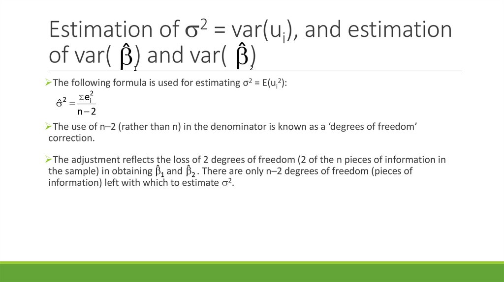
The following formula is used for estimating σ2 = E(ui2):
2
e
2
ˆ i
n 2
The use of n–2 (rather than n) in the denominator is known as a ‘degrees of freedom’
correction.
The adjustment reflects the loss of 2 degrees of freedom (2 of the n pieces of information in
the sample) in obtaining ̂1 and ̂2 . There are only n–2 degrees of freedom (pieces of
information) left with which to estimate 2.

23.

2
Estimation of = var(ui), and estimation
of var( ̂ ) and var( ̂ )
1
2
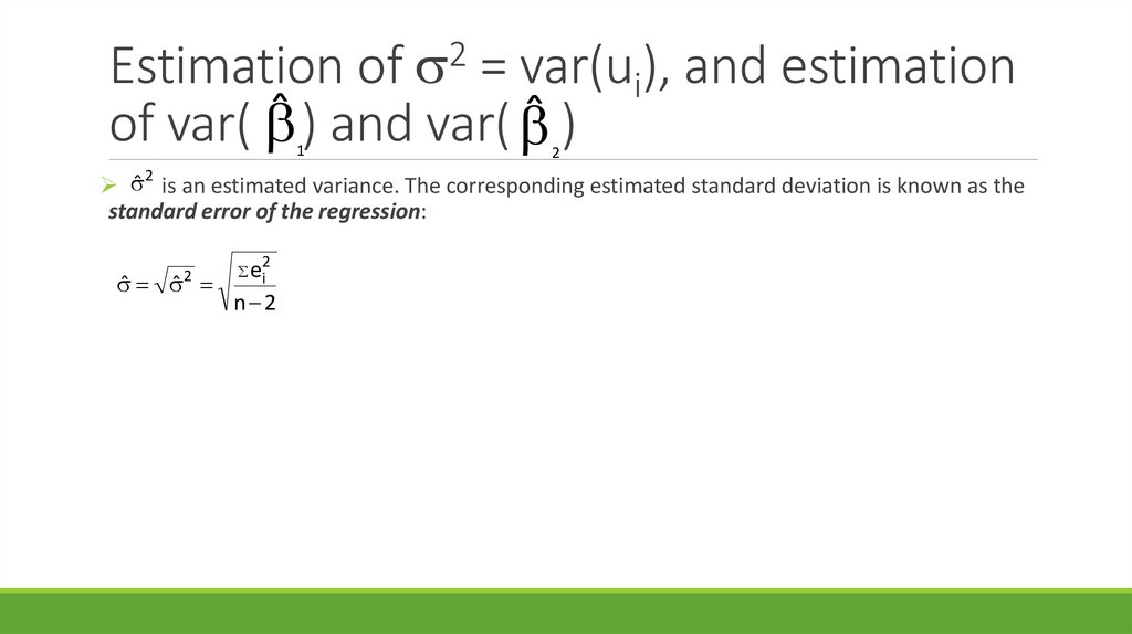
̂ is an estimated variance. The corresponding estimated standard deviation is known as the
standard error of the regression:
2
e2i
ˆ
ˆ
n 2
2

24.

2
Estimation of = var(ui), and estimation
of var( ̂ ) and var( ̂)
1
2
The expression for the estimated variance of ̂2 is:
2
ˆ
vâr( ˆ 2 )
2
(x x )
i
The corresponding standard deviation is known as the standard error of ̂2 :
se( ˆ 2 ) vâr( ˆ 2 )
N.B. This result is used for statistical inference: using the sample estimate ( ̂2) to test a
hypothesis about 2. There are equivalent results for ̂1

25.

The two-variable linear regression
model: Statistical inference
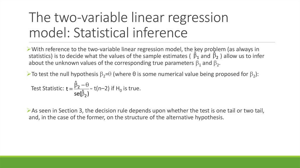
With reference to the two-variable linear regression model, the key problem (as always in
statistics) is to decide what the values of the sample estimates ( ̂1 and ̂2 ) allow us to infer
about the unknown values of the corresponding true parameters 1 and 2.
To test the null hypothesis 2= (where θ is some numerical value being proposed for 2):
ˆ 2
Test Statistic: t
̴ t(n–2) if H0 is true.
ˆ
se( 2 )
As seen in Section 3, the decision rule depends upon whether the test is one tail or two tail,
and, in the case of the former, on the structure of the alternative hypothesis.

26.

The two-variable linear regression
model: Statistical inference
The procedures are as follows (significance level: =0.05):
One-tail tests:
(a)
Test H0: 2= against H0: 2>
Decision rule: Accept H0 if t ≤ t0.05
Reject H0 if t > t0.05
(b)
Test H0: 2= against H0: 2<
Decision rule: Accept H0 if t ≥ –t0.05
Reject H0 if t < –t0.05

27.

The two-variable linear regression
model: Statistical inference
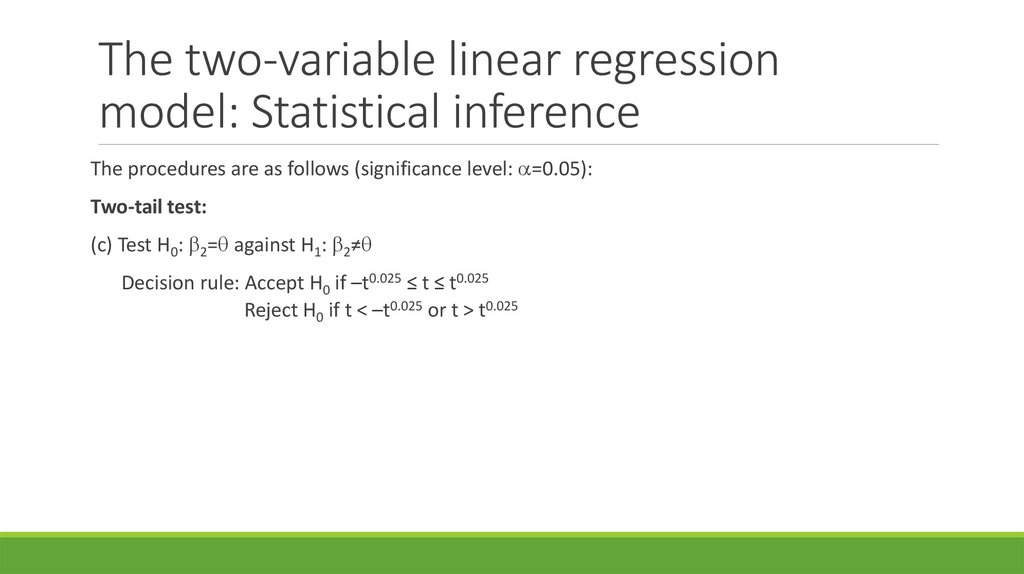
The procedures are as follows (significance level: =0.05):
Two-tail test:
(c) Test H0: 2= against H1: 2≠
Decision rule: Accept H0 if –t0.025 ≤ t ≤ t0.025
Reject H0 if t < –t0.025 or t > t0.025

28.

The two-variable linear regression
model: Statistical inference
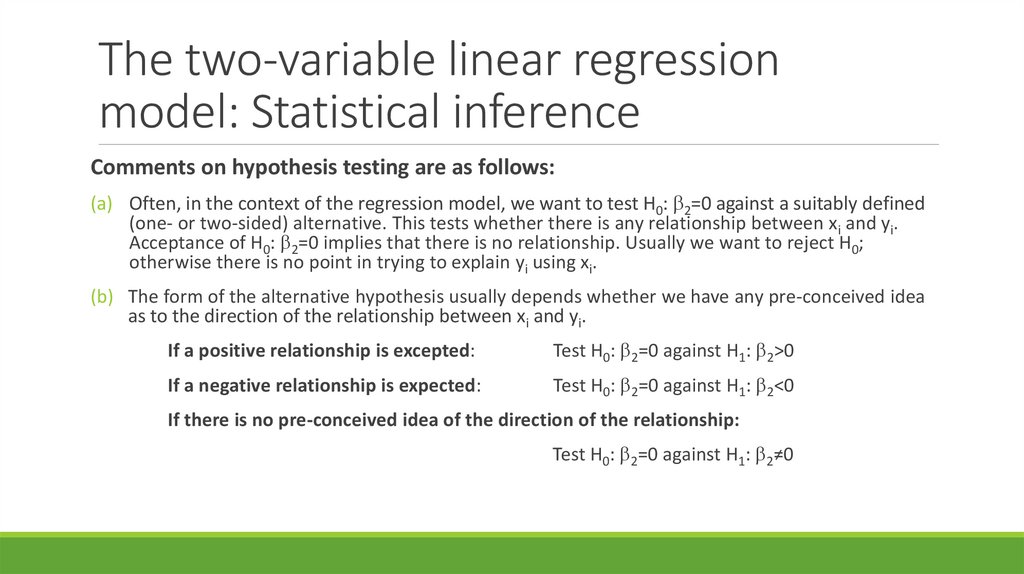
Comments on hypothesis testing are as follows:
(a) Often, in the context of the regression model, we want to test H0: 2=0 against a suitably defined
(one- or two-sided) alternative. This tests whether there is any relationship between xi and yi.
Acceptance of H0: 2=0 implies that there is no relationship. Usually we want to reject H0;
otherwise there is no point in trying to explain yi using xi.
(b) The form of the alternative hypothesis usually depends whether we have any pre-conceived idea
as to the direction of the relationship between xi and yi.
If a positive relationship is excepted:
Test H0: 2=0 against H1: 2>0
If a negative relationship is expected:
Test H0: 2=0 against H1: 2<0
If there is no pre-conceived idea of the direction of the relationship:
Test H0: 2=0 against H1: 2≠0

29.

The two-variable linear regression
model: Statistical inference
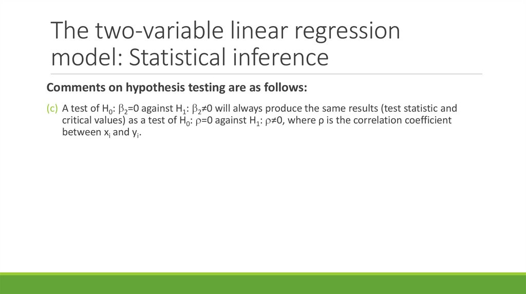
Comments on hypothesis testing are as follows:
(c) A test of H0: 2=0 against H1: 2≠0 will always produce the same results (test statistic and
critical values) as a test of H0: =0 against H1: ≠0, where ρ is the correlation coefficient
between xi and yi.

30.

Ordinary Least Squares estimation of 1
and 2
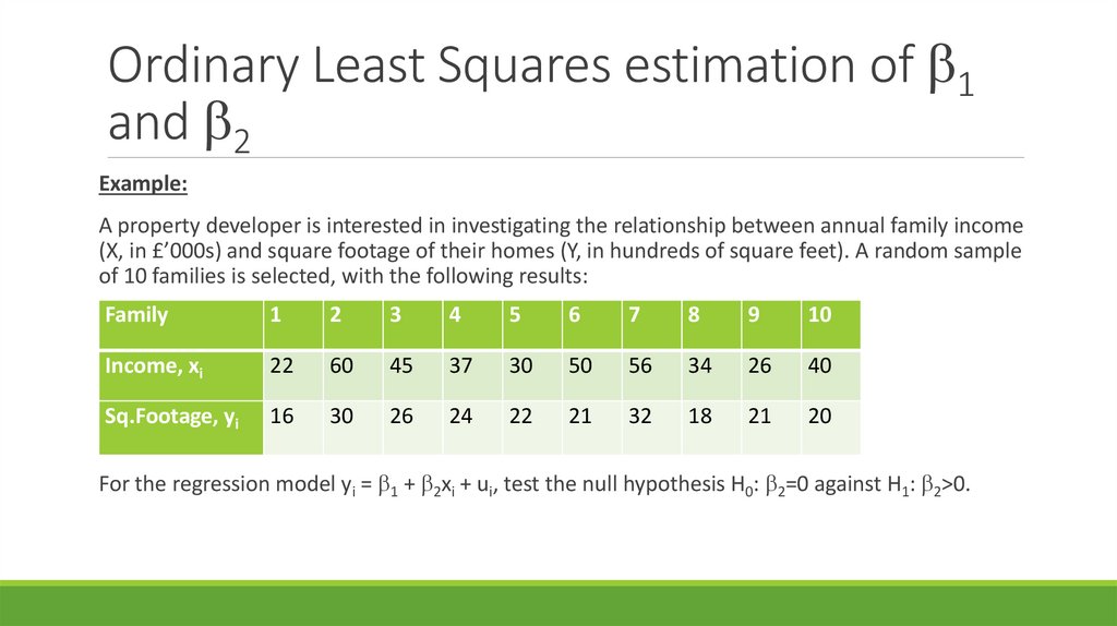
Example:
A property developer is interested in investigating the relationship between annual family income
(X, in £’000s) and square footage of their homes (Y, in hundreds of square feet). A random sample
of 10 families is selected, with the following results:
Family
1
2
3
4
5
6
7
8
9
10
Income, xi
22
60
45
37
30
50
56
34
26
40
Sq.Footage, yi
16
30
26
24
22
21
32
18
21
20
For the regression model yi = 1 + 2xi + ui, test the null hypothesis H0: 2=0 against H1: 2>0.

31.

Ordinary Least Squares estimation of 1
and 2
Solution:

32.

Ordinary Least Squares estimation of 1
and 2
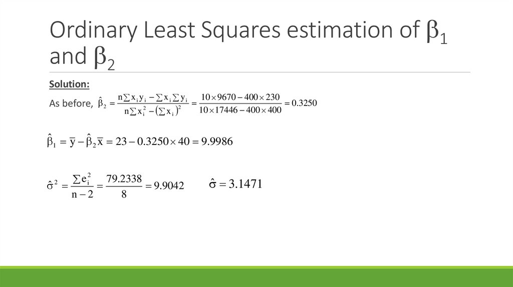
Solution:
As before, ˆ 2
n x i yi x i yi
n x i2 x i
2
10 9670 400 230
0.3250
10 17446 400 400
ˆ 1 y ˆ 2 x 23 0.3250 40 9.9986
79.2338
ei
ˆ
9.9042
n 2
8
2
2
ˆ 3.1471

33.

Ordinary Least Squares estimation of 1
and 2
Solution:
2
Using ( x i x ) 1446
2
ˆ
9.9042
vâr( ˆ 2 )
0.006849
2
1446
(x i x)
se( ˆ 2 ) 0.006849 0.08276

34.

Ordinary Least Squares estimation of 1
and 2
Solution:

35.

Ordinary Least Squares estimation of 1
and 2
Solution:
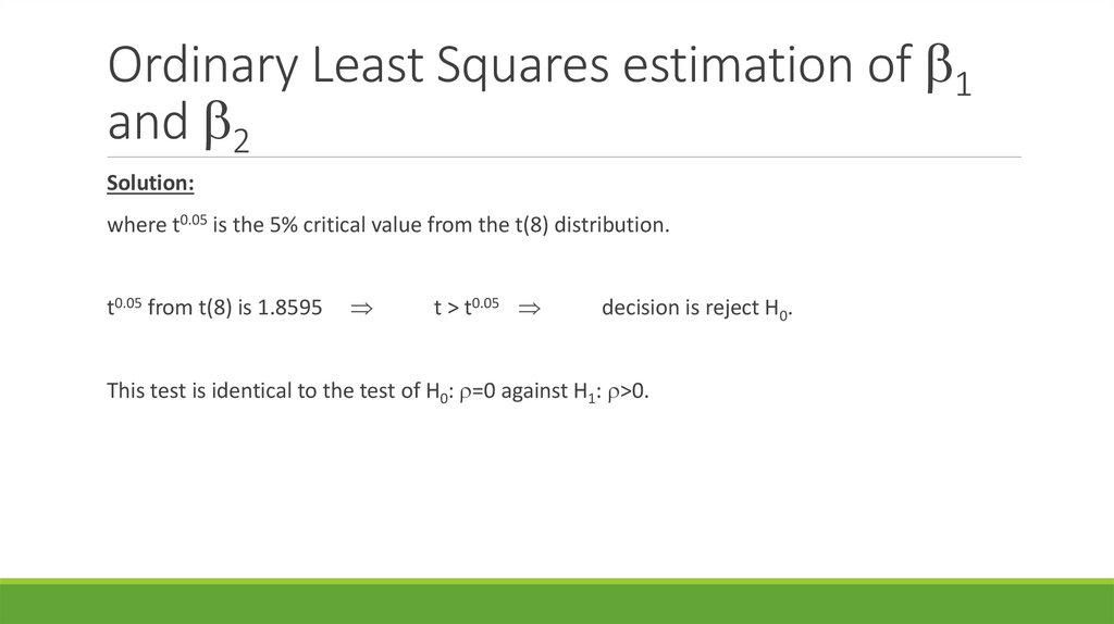
where t0.05 is the 5% critical value from the t(8) distribution.
t0.05 from t(8) is 1.8595
t > t0.05
decision is reject H0.
This test is identical to the test of H0: =0 against H1: >0.

36.

MS Excel
To run a regression on Excel, click on the Data tab, then Data Analysis, then Regression.
For this to work, the Analysis ToolPak must be installed (see Panopto of the lecture for details on
how to set the following up and run the regression):
Click on ‘File’
Choose ‘Options’
Choose ‘Add-Ins’ and ‘Manage Excel Add-Ins’
Tick ‘Analysis ToolPak’ option

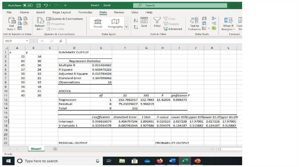
37.

38.

Regression analysis: Summary
Linear regression model: used to investigate causal relationships between two or more
variables.
Independent/explanatory variable, xi: determined exogenously (i.e. outside the model).
Variable thought to be responsible for the change in a model.
Dependent variable, yi: determined endogenously (i.e. explained/partly explained by the
independent/explanatory variable). Variable we are seeking to explain by a model.

39.

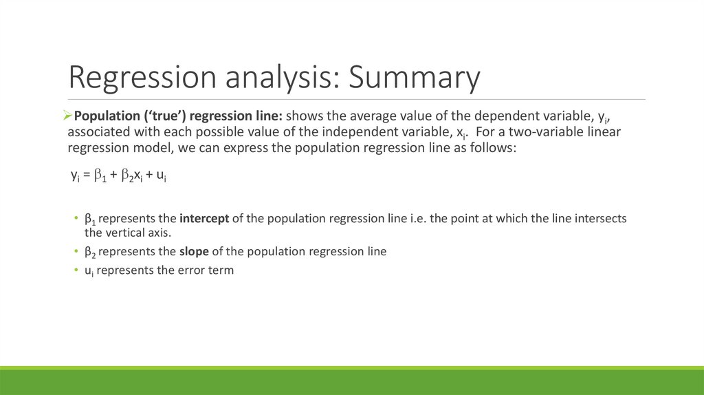
Regression analysis: Summary
Population (‘true’) regression line: shows the average value of the dependent variable, yi,
associated with each possible value of the independent variable, xi. For a two-variable linear
regression model, we can express the population regression line as follows:
yi = 1 + 2xi + ui
• β1 represents the intercept of the population regression line i.e. the point at which the line intersects
the vertical axis.
• β2 represents the slope of the population regression line
• ui represents the error term

40.

Regression analysis: Summary
Sample (‘estimated’) regression line: we usually take a random sample of n observations of the
dependent and independent variable in order to obtain estimates of β1, β2 and σ2. The sample
regression line shows the average value of the dependent variable, yi, associated with each
value of the independent variable, xi, for the sample of n observations. For a two-variable
regression model, we can express the sample regression line as follows:
y i ˆ 1 ˆ 2x i ei
• ̂1 represents the sample estimator of β1.
• ̂2 represents the sample estimator of β2.
• ei represents the estimated error term or residual, and is the sample estimator of ui

41.

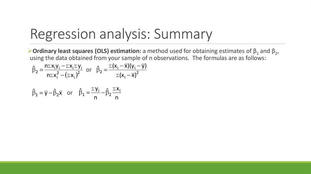
Regression analysis: Summary
Ordinary least squares (OLS) estimation: a method used for obtaining estimates of β1 and β2,
using the data obtained from your sample of n observations. The formulas are as follows:
n x iy i x i y i
ˆ 2 (x i x)(y i y)
or
ˆ 2
2
(x x )
n x 2i x i 2
i
ˆ 1 y ˆ 2 x or ˆ 1 y i ˆ 2 x i
n
n

42.

Regression analysis: Summary
Standard error of the regression: An estimated standard deviation. The formula is as follows:
e2i
ˆ
ˆ
n 2
2
Estimated variance of ̂2 : The formula is as follows:
2
ˆ
vâr( ˆ 2 )
2
(x x )
i

43.

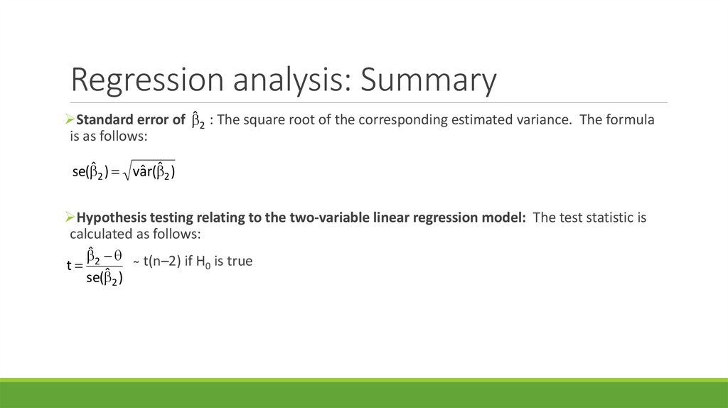
Regression analysis: Summary
Standard error of ̂2 : The square root of the corresponding estimated variance. The formula
is as follows:
se( ˆ 2 ) vâr( ˆ 2 )
Hypothesis testing relating to the two-variable linear regression model: The test statistic is
calculated as follows:
ˆ 2 ̴ t(n–2) if H is true
0
t
ˆ
se( 2 )

44.

Readings
Curwin, J., Slater, R. and Eadson, D. (2013). Quantitative Methods for Business Decisions, 7th ed.
Hampshire: Cengage.
o Chapters 15, 16
Newbold, P., Carlson, W.L. and Thorne, B. (2013). Statistics for Business and Economics, 8th ed.
Harlow: Pearson.
o Chapters 11, 12