The Simple Regression Model

1.

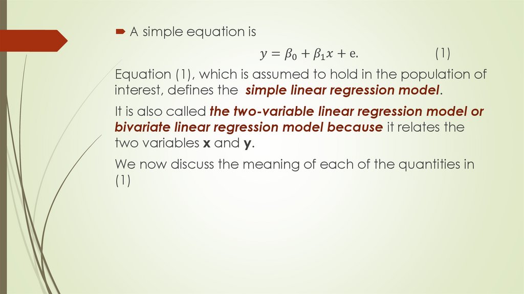
The Simple Regression Model

2.

In every regression study there is a single variable that
we are trying to explain or predict, called the
dependent variable (also called the response variable
or the target variable).
To help explain or predict the dependent variable, we
use one or more explanatory variables (also called
independent variables or predictor variables).
If there is a single explanatory variable, the analysis is
called simple regression.
If there are several explanatory variables, it is called
multiple regression

3.

The dependent (or response or target) variable
is the single variable being explained by the
regression. The explanatory (or independent or
predictor) variables are used to explain the
dependent variable

4.

A simple regression analysis includes a single
explanatory variable, whereas multiple
regression can include any number of
explanatory variables.

5.

SCATTERPLOTS: GRAPHING
RELATIONSHIPS
A good way to begin any regression analysis is to draw
one or more scatterplots.
A scatterplot is a graphical plot of two variables, an X
and a Y.
If there is any relationship between the two variables, it is
usually apparent from the scatterplot

6.

Example
Pharmex is a chain of drugstores that operates around
the country.
To see how effective its advertising and other
promotional activities are, the company has collected
data from 50 randomly selected metropolitan regions. In
each region it has compared its own promotional
expenditures and sales to those of the leading
competitor in the region over the past year.

7.

There are two variables:
■ Promote: Pharmex’s promotional expenditures as a
percentage of those of the leading competitor
■ Sales: Pharmex’s sales as a percentage of those of the
leading competitor

8.

Note that each of these variables is an index, not a
dollar amount.
For example, if Promote equals 95 for some region, this
indicates that Pharmex’s promotional expenditures in
that region are 95% as large as those for the leading
competitor in that region.

9.

The company expects that there is a positive relationship
between these two variables, so that regions with
relatively larger expenditures have relatively larger sales.
However, it is not clear what the nature of this
relationship is.
What type of relationship, if any, is apparent from a
scatterplot?

10.

If it were perfect, a given value of Promote would
prescribe the value of Sales exactly.
For example, there are five regions with promotional
values of 96 but all of them have different sales values.
So the scatterplot indicates that while the variable
Promote is helpful for predicting Sales, it does not lead to
perfect predictions.

11.

This scatterplot indicates that there is indeed a positive
relationship between Promote and Sales—the points
tend to rise from bottom left to top right—but the
relationship is not perfect.

12.

Outliers
Scatterplots are especially useful for identifying outliers,
observations that lie outside the typical pattern of points.
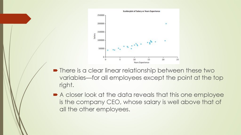
The scatterplot in Figure shows annual salaries versus
years of experience for a sample of employees at a
particular company.

13.

There is a clear linear relationship between these two
variables—for all employees except the point at the top
right.
A closer look at the data reveals that this one employee
is the company CEO, whose salary is well above that of
all the other employees.

14.

An outlier is an observation that falls outside of
the general pattern of the rest of the
observations.

15.

Although scatterplots are good for detecting outliers,
they do not necessarily indicate what you ought to do
about any outliers you find.
This depends entirely on the particular situation.
If you are attempting to investigate the salary structure
for typical employees at a company, then you should
probably not include the company CEO.

16.

First, the CEO’s salary is not determined in the same way
as the salaries for typical employees.
Second, if you do include the CEO in the analysis, it can
greatly distort the results for the mass of typical
employees.
In other situations, however, it might not be appropriate
to eliminate outliers just to make the analysis come out
more nicely.

17.

It is difficult to generalize about the treatment of outliers,
but the following points are worth noting.
■ If an outlier is clearly not a member of the population
of interest, then it is probably best to delete it from the
analysis. This is the case for the company CEO in Figure.
■ If it isn’t clear whether outliers are members of the
relevant population, you can run the regression analysis
with them and again without them. If the results are
practically the same in both cases, then it is probably
best to report the results with the outliers included.
Otherwise, you can report both sets of results with a
verbal explanation of the outliers

18.

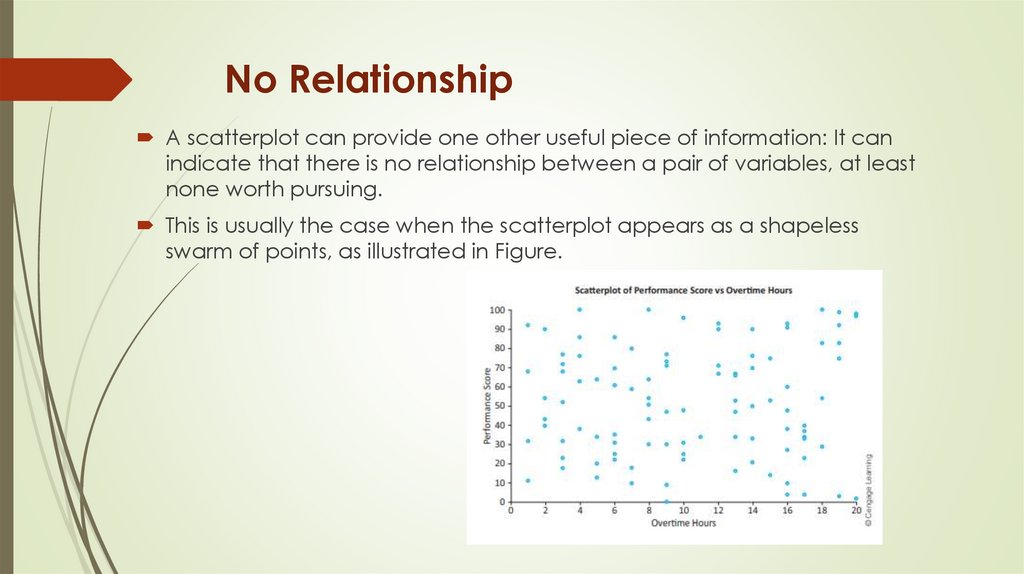
No Relationship
A scatterplot can provide one other useful piece of information: It can
indicate that there is no relationship between a pair of variables, at least
none worth pursuing.
This is usually the case when the scatterplot appears as a shapeless
swarm of points, as illustrated in Figure.

19.

Here the variables are an employee performance score
and the number of overtime hours worked in the
previous month for a sample of employees.
There is virtually no hint of a relationship between these
two variables in this plot, and if these are the only two
variables in the data set, the analysis can stop right here.

20.

CORRELATIONS: INDICATORS OF LINEAR
RELATIONSHIPS
Scatterplots provide graphical indications of
relationships, whether they are linear, nonlinear, or
essentially nonexistent.
Correlations are numerical summary measures that
indicate the strength of linear relationships between
pairs of variables.
A correlation between a pair of variables is a single
number that summarizes the information in a scatterplot.
A correlation can be very useful, but it has an important
limitation: It measures the strength of linear relationships
only.

21.

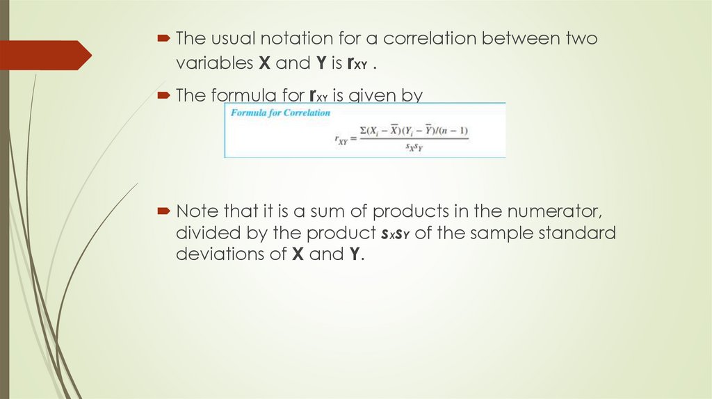
The usual notation for a correlation between two
variables X and Y is rXY .
The formula for rXY is given by
Note that it is a sum of products in the numerator,
divided by the product sXsY of the sample standard
deviations of X and Y.

22.

The numerator of Equation is also a measure of
association between two variables X and Y, called the
covariance between X and Y.
Like a correlation, a covariance is a single number that
measures the strength of the linear relationship between
two variables.
By looking at the sign of the covariance or correlation—
plus or minus—you can tell whether the two variables
are positively or negatively related.
The drawback to a covariance, however, is that its
magnitude depends on the units in which the variables
are measured.

23.

All correlations are between −1 and +1, inclusive.
The sign of a correlation, plus or minus, determines
whether the linear relationship between two variables is
positive or negative.
In this respect, a correlation is just like a covariance.
However, the strength of the linear relationship between
the variables is measured by the absolute value, or
magnitude, of the correlation.
The closer this magnitude is to 1, the stronger the linear
relationship is.

24.

A correlation equal to 0 or near 0 indicates practically
no linear relationship.
A correlation with magnitude close to 1, on the other
hand, indicates a strong linear relationship.
At the extreme, a correlation equal to −1 or +1 occurs
only when the linear relationship is perfect—that is, when
all points in the scatterplot lie on a straight line.

25.

Least Squares Estimation
The least squares line is the line that minimizes the sum of
the squared residuals. It is the line quoted in regression
outputs

26.

A simple equation is