


 economics
Similar presentations:


")


Tutorial 10. The Open Economy: the Mundell-Fleming Model
1.
Webster UniversityTutorial 10. The Open Economy:
the Mundell-Fleming Model
slide 1
2.
Question 1. Mundell-Fleming ModelExplain by making use of MF model briefly (2 or 3 sentences) why
a monetary contraction for a small open economy under fixed
exchange rates will have no effect on real income.
slide 2
3.
Question 1. Mundell-Fleming ModelAnswer:
A monetary contraction shifts the LM* curve to the left, putting
downward pressure on the exchange rate. However, the central
bank is committed to the original rate – people will then sell the
central bank foreign currency and buy domestic currency. This
will then INCREASE the money supply – in fact the money supply
returns to precisely what it was before, and thus output does not
get affected.
slide 3
4.
Question 2. Mundell-Fleming ModelIf a small open economy with a flexible exchange rate is
experiencing a recession, what will automatically happen over
time to its trade balance, foreign exchange rate, and national
output? Illustrate graphically.
slide 4
5.
Question 2. Mundell-Fleming ModelAnswer:
Say that Y(LR) is the long run
output for the economy, while Y1 is
where the economy is right now.
Then, what must happen is
PRICES WILL FALL – this of
course means that real money
balances rise, implying a rightward
shift in the LM* curve.
Note that this also implies a
decrease in the real exchange rate.
slide 5
6.
Question 3. Mundell-Fleming Model: FiscalPolicy under floating exchange rate regime
In the Mundell–Fleming model, what happens to the exchange
rate, aggregate income, and trade balance if an increase in taxes
occurs?
slide 6
7.
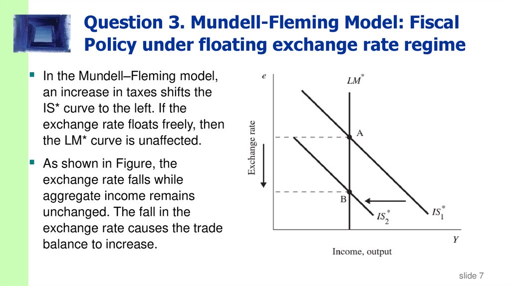
Question 3. Mundell-Fleming Model: FiscalPolicy under floating exchange rate regime
In the Mundell–Fleming model,
an increase in taxes shifts the
IS* curve to the left. If the
exchange rate floats freely, then
the LM* curve is unaffected.
As shown in Figure, the
exchange rate falls while
aggregate income remains
unchanged. The fall in the
exchange rate causes the trade
balance to increase.
slide 7
8.
Question 4. Mundell-Fleming Model: FiscalPolicy under fixed exchange rate regime
In the Mundell–Fleming model, what happens to the aggregate
income, and trade balance if an increase in taxes occurs?
slide 8
9.
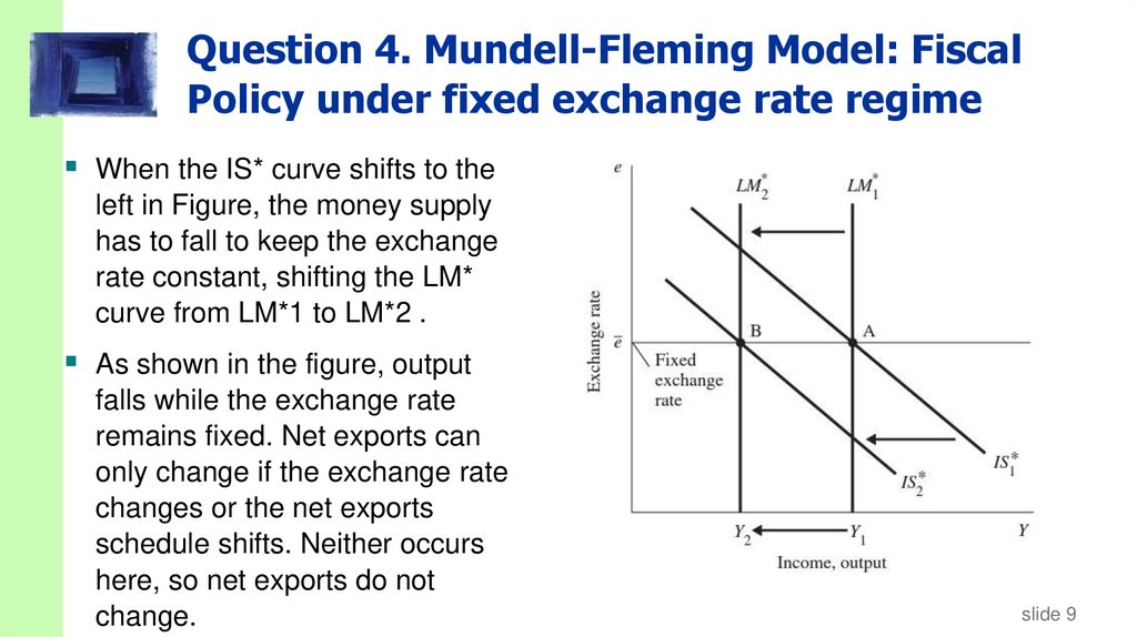
Question 4. Mundell-Fleming Model: FiscalPolicy under fixed exchange rate regime
When the IS* curve shifts to the
left in Figure, the money supply
has to fall to keep the exchange
rate constant, shifting the LM*
curve from LM*1 to LM*2 .
As shown in the figure, output
falls while the exchange rate
remains fixed. Net exports can
only change if the exchange rate
changes or the net exports
schedule shifts. Neither occurs
here, so net exports do not
change.
slide 9
10.
Question 5. Mundell-Fleming Model: FiscalPolicy effectiveness
From the answers to the questions 3 and 4, what we may
conclude about fiscal policy effectiveness: is it effective that under
fixed exchange rates or under floating exchange rates?
slide 10
11.
Question 5. Mundell-Fleming Model: FiscalPolicy effectiveness
From the answers to the questions 3 and 4, we conclude that in
an open economy, fiscal policy is effective at influencing output
under fixed exchange rates but ineffective under floating
exchange rates.
slide 11
12.
Question 6. Mundell-Fleming Model: MonetaryPolicy under floating exchange rate regime
In the Mundell–Fleming model, what happens to the exchange
rate, aggregate income, and trade balance if a reduction in the
money supply occurs?
slide 12
13.
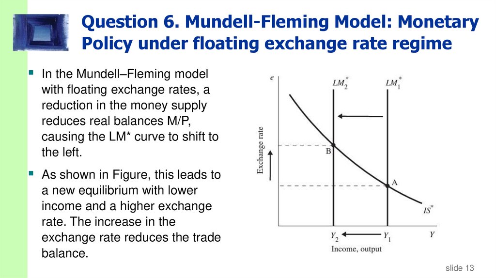
Question 6. Mundell-Fleming Model: MonetaryPolicy under floating exchange rate regime
In the Mundell–Fleming model
with floating exchange rates, a
reduction in the money supply
reduces real balances M/P,
causing the LM* curve to shift to
the left.
As shown in Figure, this leads to
a new equilibrium with lower
income and a higher exchange
rate. The increase in the
exchange rate reduces the trade
balance.
slide 13
14.
Question 7. Mundell-Fleming Model: MonetaryPolicy under fixed exchange rate regime
In the Mundell–Fleming model, what happens to the aggregate
income, and trade balance if a reduction in the money supply
occurs?
slide 14
15.
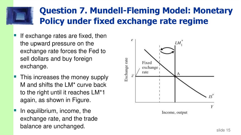
Question 7. Mundell-Fleming Model: MonetaryPolicy under fixed exchange rate regime
If exchange rates are fixed, then
the upward pressure on the
exchange rate forces the Fed to
sell dollars and buy foreign
exchange.
This increases the money supply
M and shifts the LM* curve back
to the right until it reaches LM*1
again, as shown in Figure.
In equilibrium, income, the
exchange rate, and the trade
balance are unchanged.
slide 15
16.
Question 8. Mundell-Fleming Model: MonetaryPolicy effectiveness
From the answers to the questions 3 and 4, what we may
conclude about monetary policy effectiveness: is it effective that
under fixed exchange rates or under floating exchange rates?
slide 16
17.
Question 8. Mundell-Fleming Model: MonetaryPolicy under floating exchange rate regime
From the answers to the questions 3 and 4, we conclude that in
an open economy, monetary policy is effective at influencing
output under floating exchange rates but impossible under fixed
exchange rates.
slide 17
18.
Question 9. Mundell-Fleming Model: TradePolicy under floating exchange rate regime
In the Mundell–Fleming model, what happens to the exchange
rate, aggregate income, and trade balance if a removing a quota
on imported cars occurs?
slide 18
19.
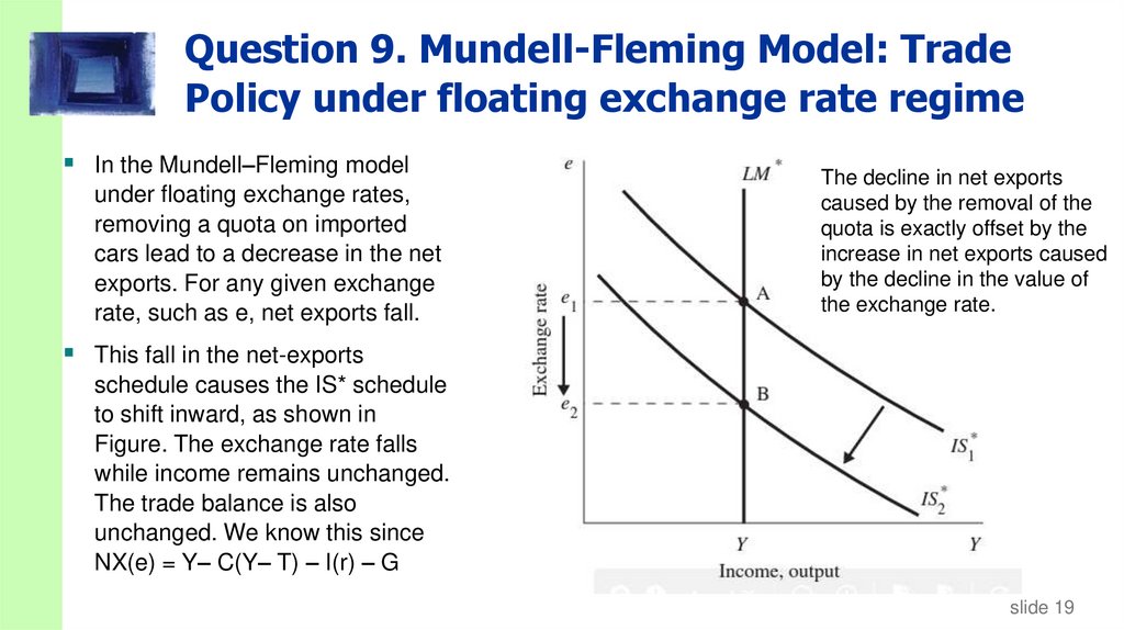
Question 9. Mundell-Fleming Model: TradePolicy under floating exchange rate regime
In the Mundell–Fleming model
under floating exchange rates,
removing a quota on imported
cars lead to a decrease in the net
exports. For any given exchange
rate, such as e, net exports fall.
The decline in net exports
caused by the removal of the
quota is exactly offset by the
increase in net exports caused
by the decline in the value of
the exchange rate.
This fall in the net-exports
schedule causes the IS* schedule
to shift inward, as shown in
Figure. The exchange rate falls
while income remains unchanged.
The trade balance is also
unchanged. We know this since
NX(e) = Y– C(Y– T) – I(r) – G
slide 19
20.
Question 10. Mundell-Fleming Model: TradePolicy under fixed exchange rate regime
In the Mundell–Fleming model, what happens to the exchange
rate, aggregate income, and trade balance if a removing a quota
on imported cars occurs?
slide 20
21.
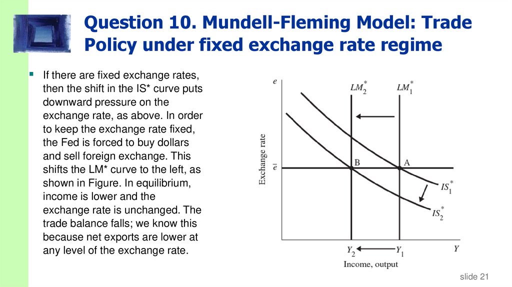
Question 10. Mundell-Fleming Model: TradePolicy under fixed exchange rate regime
If there are fixed exchange rates,
then the shift in the IS* curve puts
downward pressure on the
exchange rate, as above. In order
to keep the exchange rate fixed,
the Fed is forced to buy dollars
and sell foreign exchange. This
shifts the LM* curve to the left, as
shown in Figure. In equilibrium,
income is lower and the
exchange rate is unchanged. The
trade balance falls; we know this
because net exports are lower at
any level of the exchange rate.
slide 21
22.
Question 11. What does the impossibletrinity say?
slide 22
23.
Question 11. What does the impossibletrinity say?
The impossible trinity states that it is impossible for a nation to
have free capital flows, a fixed exchange rate, and independent
monetary policy. In other words, you can only have two of the
three. If you want free capital flows and an independent monetary
policy, then you cannot also peg the exchange rate. If you want a
fixed exchange rate and free capital flows, then you cannot have
independent monetary policy. If you want to have independent
monetary policy and a fixed exchange rate, then you need to
restrict capital flows.
slide 23
24.
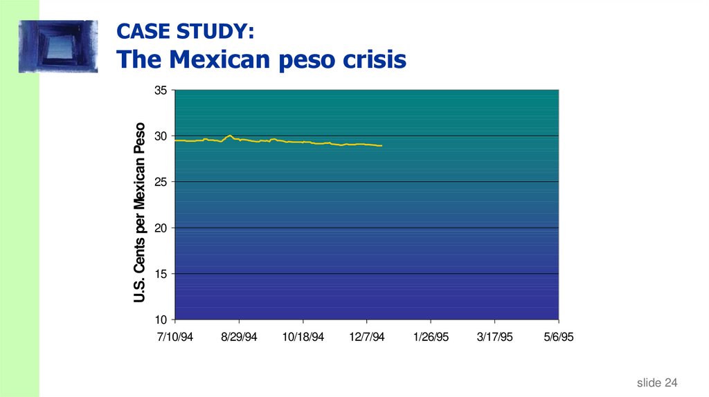
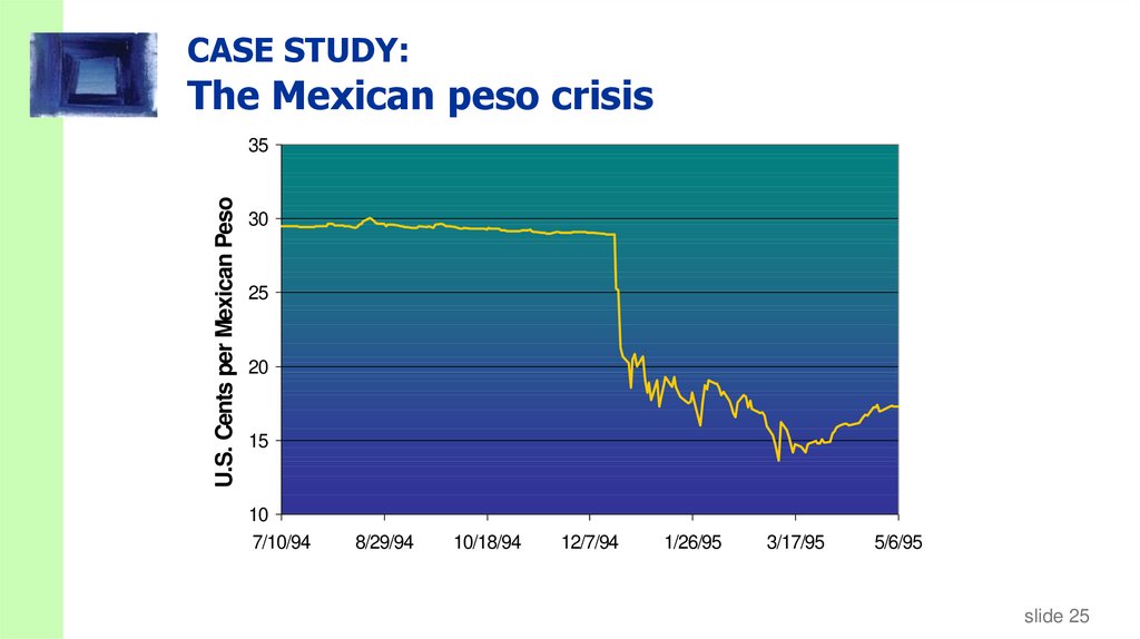
CASE STUDY:The Mexican peso crisis
U.S. Cents per Mexican Peso
35
30
25
20
15
10
7/10/94
8/29/94
10/18/94
12/7/94
1/26/95
3/17/95
5/6/95
slide 24
25.
CASE STUDY:The Mexican peso crisis
U.S. Cents per Mexican Peso
35
30
25
20
15
10
7/10/94
8/29/94
10/18/94
12/7/94
1/26/95
3/17/95
5/6/95
slide 25
26.
The Peso crisis didn’t just hurt MexicoU.S. goods more expensive to Mexicans
U.S. firms lost revenue
Hundreds of bankruptcies along
U.S.-Mexican border
Mexican assets worth less in dollars
Reduced wealth of millions of U.S. citizens
slide 26
27.
Understanding the crisisIn the early 1990s, Mexico was an attractive place
for foreign investment.
During 1994, political developments caused an
increase in Mexico’s risk premium ( ):
peasant uprising in Chiapas
assassination of leading presidential candidate
Another factor:
The Federal Reserve raised U.S. interest rates
several times during 1994 to prevent U.S. inflation.
( r* > 0)
slide 27
28.
Understanding the crisisThese events put downward pressure on the peso.
Mexico’s central bank had repeatedly promised foreign investors that
it would not allow the peso’s value to fall,
so it bought pesos and sold dollars to
“prop up” the peso exchange rate.
Doing this requires that Mexico’s central bank have adequate
reserves of dollars.
Did it?
slide 28
29.
Dollar reserves of Mexico’s central bankDecember 1993 ……………… $28 billion
August 17, 1994 ……………… $17 billion
December 1, 1994 …………… $ 9 billion
December 15, 1994 ………… $ 7 billion
During 1994, Mexico’s central bank hid the
fact that its reserves were being depleted.
slide 29
30.
the disasterDec. 20: Mexico devalues the peso by 13%
(fixes e at 25 cents instead of 29 cents)
Investors are SHOCKED! – they had no idea
Mexico was running out of reserves.
, investors dump their Mexican assets and
pull their capital out of Mexico.
Dec. 22: central bank’s reserves nearly gone.
It abandons the fixed rate and lets e float.
In a week, e falls another 30%.
slide 30
31.
The rescue package1995: U.S. & IMF set up $50b line of credit to provide loan
guarantees to Mexico’s govt.
This helped restore confidence in Mexico, reduced the risk
premium.
After a hard recession in 1995, Mexico began a strong recovery
from the crisis.
slide 31
32.
CASE STUDY:The Southeast Asian crisis 1997-98
Problems in the banking system eroded
international confidence in SE Asian economies.
Risk premiums and interest rates rose.
Stock prices fell as foreign investors sold assets
and pulled their capital out.
Falling stock prices reduced the value of collateral
used for bank loans, increasing default rates,
which exacerbated the crisis.
Capital outflows depressed exchange rates.
slide 32
33.
Data on the SE Asian crisisexchange rate
stock market nominal GDP
% change from % change from
% change
7/97 to 1/98
7/97 to 1/98
1997-98
Indonesia
-59.4%
-32.6%
-16.2%
Japan
-12.0%
-18.2%
-4.3%
Malaysia
-36.4%
-43.8%
-6.8%
Singapore
-15.6%
-36.0%
-0.1%
S. Korea
-47.5%
-21.9%
-7.3%
Taiwan
-14.6%
-19.7%
n.a.
Thailand
-48.3%
-25.6%
-1.2%
U.S.
n.a.
2.7%
2.3%
slide 33
34.
CASE STUDY:The Chinese Currency Controversy
1995-2005: China fixed its exchange rate at 8.28
yuan per dollar, and restricted capital flows.
Many observers believed that the yuan was
significantly undervalued, as China was
accumulating large dollar reserves.
U.S. producers complained that China’s cheap
yuan gave Chinese producers an unfair advantage.
President Bush asked China to let its currency float;
Others in the U.S. wanted tariffs on Chinese goods.
slide 34
35.
CASE STUDY:The Chinese Currency Controversy
If China lets the yuan float, it may indeed
appreciate.
However, if China also allows greater capital
mobility, then Chinese citizens may start moving
their savings abroad.
Such capital outflows could cause the yuan to
depreciate rather than appreciate.
slide 35