Statistics. Data Description. Data Summarization. Numerical Measures of the Data

1. Chapter Three: Data Description

A
U
S
T
N
3-1
Chapter Three:
Data Description
Data Summarization
Numerical Measures of the Data
Statistics103110

2. Chapter Three: Numerical Measures of the Data

A
U
S
T
N
3-2
Outline
Introduction
3-1 Measures of Central Tendency
3-2 Measures of Variation
3-3 Measures of Position
3-4 Exploratory Data Analysis
Statistics103110

3. Chapter Three: Numerical Measures of the Data

A
U
S
T
N
3-3
Objectives
1. Summarize
data using the measures of central
tendency, such as the mean, median, mode, and
midrange.
2. Describe data using the measures of variation,
such as the range, variance, and standard
deviation.
3. Identify the position of a data value in a data set
using various measures of position, such as
percentiles, and quartiles.
4. Use the techniques of exploratory data analysis,
including stem and leaf plots, box plots, and
five-number summaries to discover various
aspects of data.
Statistics103110

4. Chapter Three: Numerical Measures of the Data

A 3-1 Measures of Central tendency
U
S
T
N
We will compute two means: one for the sample and one for
a finite population of values.
The symbol X represents the sample mean
X X 2 ... + X n
X = 1
n
X
n
.
The Greek symbol represents the population
mean. The symbol is read as " mu".
N is the size of the finite population.
X 1 X 2 ... + X N
N
X
.
N
=
3-4
Statistics103110

5. Chapter Three: Numerical Measures of the Data

A
U
S
T
N
3-5
Example:- (Sample Mean
)
The ages of a random sample of seven
students at a certain school are 11, 10,
12, 13, 7, 9, 15
Find the average (Mean) age of this sample
X
X =
n
11 + 10 + 12 + 13 + 7 + 9 15
=
7
77
=
11 years.
7
Statistics103110

6. Chapter Three: Numerical Measures of the Data

A
U
S
T
N
3-6
Example:- population mean
A small company consists of the owner , the manager ,
the salesperson, and two technicians. The salaries are
listed as $5000, 2000, 1200, 900 and 900
respectively. ( Assume this is the population.)
Then the population mean will be
X
=
N
5000 + 2000 + 1200 + 900 + 900
=
5
= $2000.
Statistics103110

7. Chapter Three: Numerical Measures of the Data

A The mean for an ungrouped frequency
distributuion is given by
U
(f X)
S
X=
.
n
Here f is the frequency for the
T corresponding value of X , and n = f .
N
The Sample Mean for an Ungrouped Frequency Distribution
3-7
Statistics103110

8. Chapter Three: Numerical Measures of the Data

A
U
S
T
N
3-8
The Sample Mean for an Ungrouped
Frequency Distribution –
Example
The scores for 25 students on a 4 point
quiz are given in the table. Find the mean score.
Score
Frequency f.X
0
2
0
1
4
4
2
12
24
3
4
12
4
3
12
f X
X =
n
=
52
2.08.
25
Statistics103110

9. Chapter Three: Numerical Measures of the Data

A
U
S
T
N
3-9
The Sample Mean for a Grouped Frequency Distribution
The mean for a grouped frequency distribution is
given by :
X=
( f X
Xm
Here
m
)
n
is the corresponding class midpoint
Given the table below, find the mean.
Xm
f .X m
Class
Frequency
15.5 - 20.5
3
18
54
20.5 - 25.5
5
23
115
25.5 - 30.5
4
28
112
30.5 - 35.5
3
33
99
35.5 - 40.5
2
38
76
f X
m
54 115 112 99 76
= 456
and n = 17. So
X =
f X
m
n
456
=
26.82.
17
Statistics103110

10. Important remark :

A
U
S
T
N
Important remark :
In some situations the mean may not be representative
of the data.
As an example, the annual salaries of five vice
presidents at AVX, LLC are $90,000, $92,000, $94,000,
$98,000, and $350,000. The mean is:
Notice how the one extreme value ($350,000) pulled the
mean upward. Four of the five vice presidents earned
less than the mean, raising the question whether the
arithmetic mean value of $144,800 is typical of the
salary of the five vice presidents.

11. Properties of the mean

A
U
S
T
N
Properties of the mean
As stated, the mean is a widely used measure of central
tendency . It has several important properties.
1.
Every set of interval level and ratio level data has a mean.
2.
All the data values are included in the calculation.
3.
A set of data has only one mean, that is, the mean is unique.
4.
The mean is a useful measure for comparing two or more
populations.
5.
The sum of the deviations of each value from the mean will
always be zero, that is ( X X ) 0
6.
The mean is highly affected by extreme data .
Note: Illustrating the fifth property
Consider the set of values: 3, 8, and 4. The mean is 5.
( X X ) (3 5) (8 5) ( 4 5) 0
11

12. Chapter Three: Numerical Measures of the Data

A
U
S
T
N
3-12
Median
: The median splits the ordered data into
halves
the symbol used to denote the median is
me
Example:- The weights (in pounds) of seven army
recruits are 180, 201, 220, 191, 219, 209, and 186.
Find the median.
Arrange the data in order and select the middle point.
Data array: 180, 186, 191, 201, 209, 219, 220.
The median, = 201.
In the previous example, there was an odd number of
values in the data set. In this case it is easy to select
the middle number in the data array.
Statistics103110

13. Chapter Three: Numerical Measures of the Data

A
U
S
T
N
3-13
When there is an even number of values in the data set, the
median is obtained by taking the average of the two middle
numbers.
numbers
Example:Six customers purchased the following number of magazines:
1, 7, 3, 2, 3, 4. Find the median.
Arrange the data in order and compute the middle point.
Data array: 1, 2, 3, 3, 4, 7.
The median,
me = (3 + 3)/2 = 3.
Example:-Find the median grade of the following sample
62, 68, 71, 74, 77, 82, 84, 88, 90, 94
62, 68, 71, 74, 77
82, 84, 88, 90, 94
5 on the left
5 on the right
me= 79.5
Statistics103110

14. example

A
U
S
T
N
Find
the median grade of the following sample
of students grades :
ABADFDFABCCCFDAFDAABBFDAB
FC
Data array:
FFFFFFDDDDDCCCCBBBBBAAAAA
AA
The median grade is : C
Half of the students had at least C ( a grade less
than or equal C.
Half of the students had at most C ( a grade more
than or equal C .
The median can be determined for ordinal level
data .
14

15. Properties of the Median

A
U
S
T
N
The
major properties of the median are:
1. The median is a unique value, that is, like the mean,
there is only one median for a set of data.
2. It is not influenced by extremely large or small values
and is therefore a valuable measure of central
tendency when such values do occur.
3. It can be computed for ratio level, interval level, and
ordinal-level data.
4. Fifty percent of the observations are greater than the
median and fifty percent of the observations are less
than the median.
15

16. Chapter Three: Numerical Measures of the Data

A
U
S
T
N
3-16
Mode:- is the score that occurs most frequently (denoted by M)
Example:-
The following data represent the duration (in
days) of U.S. space shuttle voyages for the years 199294. Find the mode.
Data set: 8, 9, 9, 14, 8, 8, 10, 7, 6, 9, 7, 8, 10, 14, 11, 8, 14, 11.
Ordered set: 6, 7, 7, 8, 8, 8, 8, 8, 9, 9, 9, 10, 10, 11, 11, 14, 14, 14.
Mode = 8 days.
days
Example:- Six strains of bacteria were tested to see how
long they could remain alive outside their normal
environment. The time, in minutes, is given below. Find
the mode.
Data set: 2, 3, 5, 7, 8, 10.
There is no mode. since each data value occurs equally
with a frequency of one.
Statistics103110

17. Chapter Three: Numerical Measures of the Data

A
U
S
T
N
3-17
Example:- Eleven different automobiles were tested
at a speed of 15 mph for stopping distances. The
distance, in feet, is given below. Find the mode.
Data set: 15, 18, 18, 18, 20, 22, 24, 24, 24, 26, 26.
There are two modes (bimodal).
(bimodal) The values are 18
and 24.
24
Values
Frequency, f
15
3
20
5
25
8
30
3
35
2
Statistics103110

18. Chapter Three: Numerical Measures of the Data

A
U
S
T
N
3-18
The Mode for a Grouped Frequency Distribution –
Can be approximated by the midpoint of the modal class.
Example
Modal
Class
Statistics103110

19. Properties of the Mode

A
U
S
T
N
1.
2.
3.
4.
The mode can be found for all levels
of data (nominal, ordinal, interval,
and ratio).
The mode is not affected by
extremely high or low values.
A set of data can have more than
one mode. If it has two modes, it is
said to be bimodal.
A disadvantage is that a set of data
may not have a mode because no
value appears more than once.
19

20. Chapter Three: Numerical Measures of the Data

A
U
S
T
N
3-20
The weighted mean is used when the values in a
data set are not all equally represented.
The weighted mean of a variable X is found by
multiplying each value by its corresponding weight
and dividing the sum of the products by the sum of
the weights.
The weighted mean
w1 X 1 w2 X 2 ... wn X n
Xw =
w1 w 2 ... wn
wX
w
where w1 , w2 , ..., wn are the weights
for the values X 1 , X 2 , ..., X n .
Statistics103110

21. Chapter Three: Numerical Measures of the Data

A
U
S
T
N
3-21
Example:-
During a one hour period on a hot
Saturday afternoon a boy served fifty drinks. He sold five
drinks for $0.50, fifteen for $0.75, fifteen for $0.90, and
fifteen for $1.10. Compute the weighted mean of the
the price of the drinks :afternoon a boy served fifty
of
5($0.50) 15($0.75) 15($0.90) 15($1.15)
Xw
5 15 15 15
$44.50
$0.89
50
Statistics103110

22. Best measure of central tendency

A
U
S
T
N
Best measure of central tendency
Type of Variable
Best measure of central
tendency
Nominal
Mode
Ordinal
Median
Interval/Ratio (not skewed)
Mean
Interval/Ratio (skewed)
Median

23. Relationship between mean , median and mode and the shape of the distribution

A
U
S
T
N
Relationship between mean , median and
mode and the shape of the distribution
Symmetric – the mean =the median=the mode
Skewed left – the mean will usually be smaller than the
median
Skewed right – the mean will usually be larger than the
median
Dr.Nadia Ouakli
23

24. Chapter Three: Numerical Measures of the Data

3-2 Measures of Dispersion( variation)
o the spread or variability in the data.
Learning objectives
◦
◦
◦
◦
3-24
The
The
The
Use
range of a variable
variance of a variable
standard deviation of a variable
the Empirical Rule
Comparing two sets of data
The measures of central tendency (mean, median, mode)
measure the differences between the “average” or
“typical” values between two sets of data
The measures of dispersion in this section measure the
differences between how far “spread out” the data values
are.
Statistics103110

25. Chapter Three: Numerical Measures of the Data

Variability -- provides a quantitative measure of the degree to
which scores in a distribution are spread out or clustered
together.
o Tells how meaningful measures of central tendency are
o Help to see which scores are outliers (extreme scores)
Why do we Study Dispersion?
A direct comparison of two sets of data based only on two
measures of central tendency such as the mean and the
median can be misleading since an average does not tell us
anything about the spread of the data.
See Example 3-15 page 128 of your text book
Comparison of two outdoor paints : 6 gallons of each brand
have been tested and the data obtained show how long ( in
months) each brand will last before fading .
Brand A : 10 60 50 30 40 20
Brand B : 35 45 30 35 40 25
Calculate the mean for each brand :
3-25
Statistics103110

26. Chapter Three: Numerical Measures of the Data

Measures of dispersion are :
1.The
range ,
2.
The interquartile range ,
3.
The variance and standard deviation ,
4.
The coefficient of variation
The range (R) of a variable is the difference between the largest
data value and the smallest data value
R = highest value – lowest value.
Properties of the range
1.Only
3-26
two values are used in the calculation.
2.It
is influenced by extreme values.
3.It
is easy to compute and understand.
Statistics103110

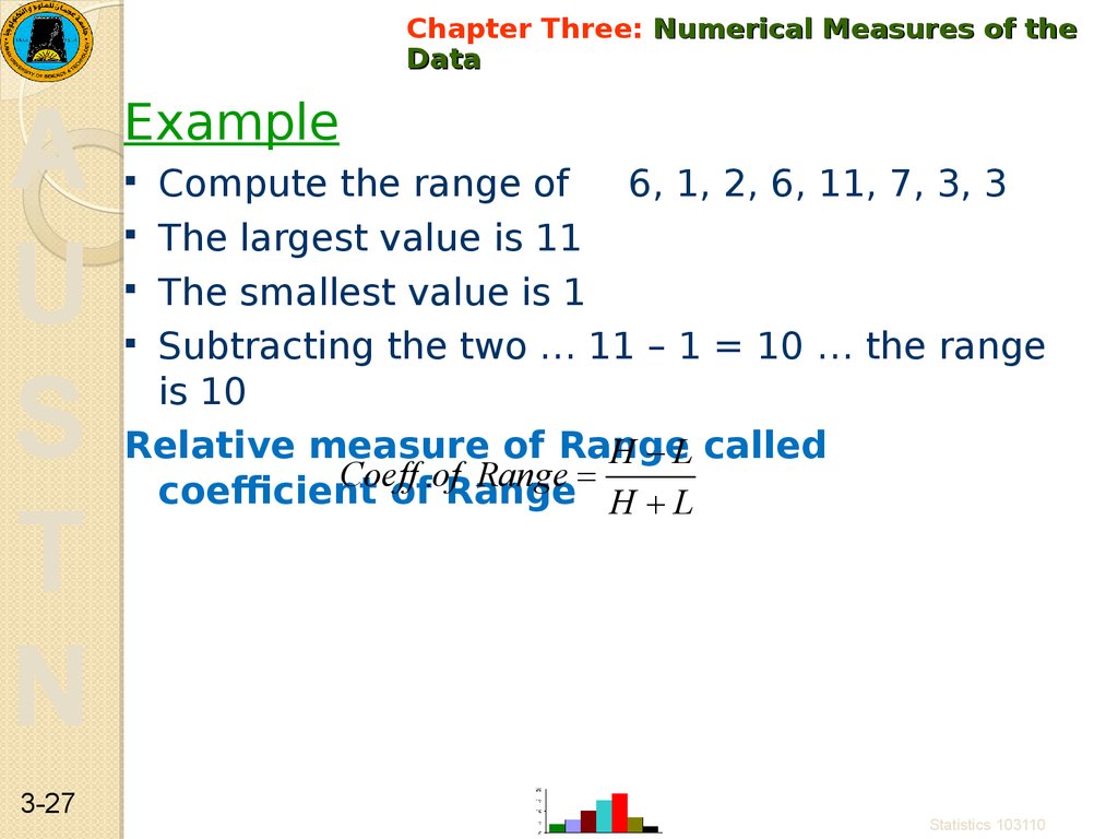
27.

Chapter Three: Numerical Measures of the
Data
A
U
S
T
N
3-27
Example
Compute the range of
6, 1, 2, 6, 11, 7, 3, 3
The largest value is 11
The smallest value is 1
Subtracting the two … 11 – 1 = 10 … the range
is 10
Relative measure of Range
H L called
Coeff
Range
coefficient
of.ofRange
H L
Statistics 103110

28. Chapter Three: Numerical Measures of the Data

The variance of a variable
The variance is based on the
deviation from the mean
( xi – μ ) for populations
( xi – x ) for samples
To treat positive differences and
negative differences, we square the
deviations
( xi – xμ )2 for populations
( xi – )2 for samples
3-28
Statistics103110

29. Chapter Three: Numerical Measures of the Data

The population variance of a variable is the sum of the squared
deviations of the data values from the mean divided by the number in the
population
where
2
(X )
2
The population variance is represented by σ2
N
X = individual value
= population mean
N = population size
i.e. the square root of the arithmetic mean of the squares of
deviations from arithmetic mean of given distribution.
Standard deviation: The square root of the variance.
3-29
2

30. Chapter Three: Numerical Measures of the Data

Properties of the variance and standard deviation
1. it is the typical or approx. average distance from the
mean
2. if it is small, then scores are clustered close to mean; if
it is large, they are scattered far from mean
3. it describes how variable or spread out the scores are.
4. it is very influenced by extreme scores
5. The measurement units of the variance are square of
the original units. While the measurement of the SD is
same as the original data
6. All values are used in the calculation.
7 . Variance and St. dev are always greater than or equal
to zero. They are equal zero only if all observations are
the same.
3-30
Statistics103110

31. Chapter Three: Numerical Measures of the Data

The sample variance
of a variable is the sum
of the squared deviations of data values from the
mean divided by one less than the number in the 2
(X - X )
sample
s2 =
The sample variance is represented by
s2
Sample standard deviation (s)
n -1
s
s2
We say that this statistic has n – 1 degrees of freedom
Example;- Find the variance and standard deviation for the
following sample: 16, 19, 15, 15, 14.
X = 16 + 19 + 15 + 15 + 14 = 79.
X2 = 162 + 192 + 152 + 152 + 142 = 1263.
Using the short cut formula ( without calculating the
mean)
( x ) 2
2
2
2
n x ( x )
x
2
s
3-31
n( n 1)
or
s2
(n 1)
n
s 3.7 1.9235
Statistics103110

32.

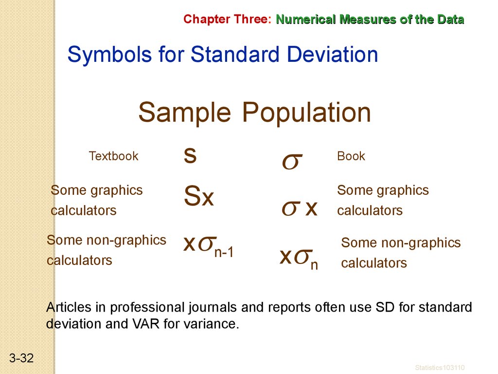
Chapter Three: Numerical Measures of the Data
Symbols for Standard Deviation
Sample Population
Textbook
Book
s
Some graphics
calculators
Some non-graphics
calculators
Sx
x n-1
x
Some graphics
calculators
x n
Some non-graphics
calculators
Articles in professional journals and reports often use SD for standard
deviation and VAR for variance.
3-32
Statistics103110

33. Chapter Three: Numerical Measures of the Data

Sample Variance for Grouped and
Ungrouped Data
For grouped data, use the class midpoints for
the observed value in the different classes.
For ungrouped data, use the same formula
with the class midpoints, Xm, replaced with
the actual observed X value.
Example:Find the variance and SD for the following
data set
2,3,4,5,2,2,2,3,2,4,3,2,5,2,3,3,4,2,5,4,4,3,3,2,
5,2
3-33
Statistics103110

34. Chapter Three: Numerical Measures of the Data

Step one put the data I ungrouped
Value (x) Frequency
f
frequency
table
f .x
f .x
x2
2
2
10
4
20
40
3
7
9
21
63
4
5
16
20
80
5
4
25
20
100
Total
26
81
283
n f x ( fx ) 2
26( 283) 812
s
n( n 1)
26( 26 1)
797
1.2262
650
2
2
3-34
s 1.2262 1.1073
Statistics103110

35. Chapter Three: Numerical Measures of the Data

Example:- find the variance and SD for the frequency distribution of
the data representing number of miles that 20 runners run during
one week
Class
5- 11
3-35
Freq. f
1
Midpoint
f .xm
8
xm
2
xm
f .xm2
8
64
64
28
196
392
11-17
2
14
17-23
3
20
60
400
1200
23-29
5
26
130
676
3380
29-35
4
32
128
1024
4096
35-41
3
38
114
1444
4332
41-47
2
44
88
1936
3872
total
20
556
17336
Statistics103110

36. Chapter Three: Numerical Measures of the Data

n f x ( fx )
2
s
2
n(n 1)
2
20(17336) 556
20(20 1)
37584
98.905
380
s 98.905 9.95
3-36
Statistics103110
2

37. Chapter Three: Numerical Measures of the Data

Interpretation and Uses of the
Standard Deviation
The standard deviation is used to
measure the spread of the data. A
small standard deviation indicates
that the data is clustered close to the
mean, thus the mean is
representative of the data. A large
standard deviation indicates that the
data are spread out from the mean
and the mean is not representative of
the data.
3-37
Statistics103110

38. Chapter Three: Numerical Measures of the Data

Coefficient of Variation :- C.V .
The relative measure of St. Dev. is the coefficient of
variation which is defined to be the standard deviation
divided by the mean. The result is expressed as a
percentage.
s
Or
C.V . .100%
C .V .
.100%
x
Important note:
The coefficient of variation should only be computed
for data measured on a ratio scale.
See the following example
3-38
Statistics103110

39. Example :

A
U
S
T
N
Example :
To
see why the coefficient of variation should not be
applied to interval level data, compare the same set of
temperatures in Celsius and Fahrenheit:
Celsius: [0, 10, 20, 30, 40]
Fahrenheit: [32, 50, 68, 86, 104]
The CV of the first set is 15.81/20 = 0.79. For the second
set (which are the same temperatures) it is 28.46/68 = 0.42
So the coefficient of variation does not have any
meaning for data on an interval scale.
39

40.

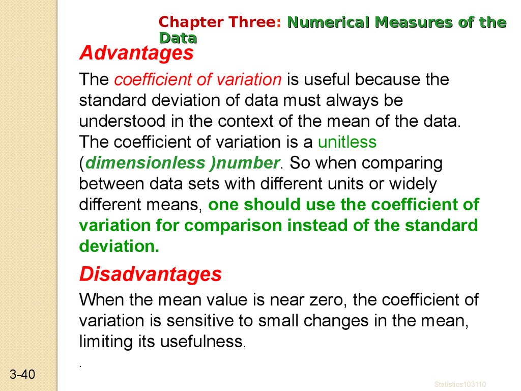
Chapter Three: Numerical Measures of the
Data
Advantages
The coefficient of variation is useful because the
standard deviation of data must always be
understood in the context of the mean of the data.
The coefficient of variation is a unitless
(dimensionless )number. So when comparing
between data sets with different units or widely
different means, one should use the coefficient of
variation for comparison instead of the standard
deviation.
Disadvantages
When the mean value is near zero, the coefficient of
variation is sensitive to small changes in the mean,
limiting its usefulness.
3-40
.
Statistics103110

41. Chapter Three: Numerical Measures of the Data

Example:- Data about the annual salary (000’s) and
age of CEO’s in a number of firms has been collected.
The means and standard deviations are as follows:
Mean
SD
Salary
404.2
220.5
Age
51.47
8.92
•Which
distribution has more dispersion? Is direct
comparison appropriate?
Salary and age are measured in different units and the means
show that there is also a significant difference in magnitude.
Direct comparison is not appropriate
Mean
SD
C.V.
Salary
404.2
220.5
54.55%
Age
51.47
8.92
17.33%
Comparing CV’s we can now see clearly that the dispersion or
variability relative to the mean is greater for CEO annual salary
than for age.
3-41
Statistics103110

42. Chapter Three: Numerical Measures of the Data

A
U
S
T
N
3-42
Measure of position:
Measures of position are used to locate the relative
position of a data value in the data set
1- Standard Scores
To compare values of different units a z-score for each
value is needed to be obtained then compared
A z-score or standard score for each value is obtained
by
For sample
z
x x
s
or
For population
z
x
The z-score represents the number SD that a data
value falls above or below the mean.
Statistics103110

43. Chapter Three: Numerical Measures of the Data

A
U
S
T
N
3-43
Standard Scores (or z-scores) specify the
exact location of a score within a
distribution relative to the mean
• The sign (- or +) tells whether the score is
above or below the mean
• The numerical value tells the distance from the
mean in terms of standard deviations
E.g., a z-score of -1.3 tells us that the raw score
fell 1.3 standard deviations below the mean.
 
Raw score is the original, untransformed score.
To make them more meaningful, raw scores can
be converted to z-scores.
Statistics103110

44. Chapter Three: Numerical Measures of the Data

A
U
S
T
N
3-44
Characteristics of Standard Scores
1. The shape of the distribution of standard scores is
the same as the shape of the distribution of raw
scores (the only thing that changes is the units on
the x-axis)
2. The mean of a set of standard scores = 0.
3. The St. deviation of a set of standard scores = 1.
4. A standard score of greater than +3 or less
than - 3 is an extreme score, or an outlier.
Statistics103110

45. Chapter Three: Numerical Measures of the Data

A
U
S
T
N
3-45
Example:- A student scored 65 on a statistics exam that
had a mean of 50 and a standard deviation of 10.
Compute the z-score.
z = (65 – 50)/10 = 1.5.
That is, the score of 65 is 1.5 standard deviations above
the mean.
Above - since the z-score is positive.
Assume that this student scored 70 on a math exam
that had a mean of 80 and a standard deviation of 5 .
Compute the z-score .
Z= ( 70-80)/5=-2
That is, the score of 70 is 2 standard deviations below
the mean.
below - since the z-score is positive.
Statistics103110

46.

Chapter Three: Numerical Measures of the
Data
A
U
S
T
N
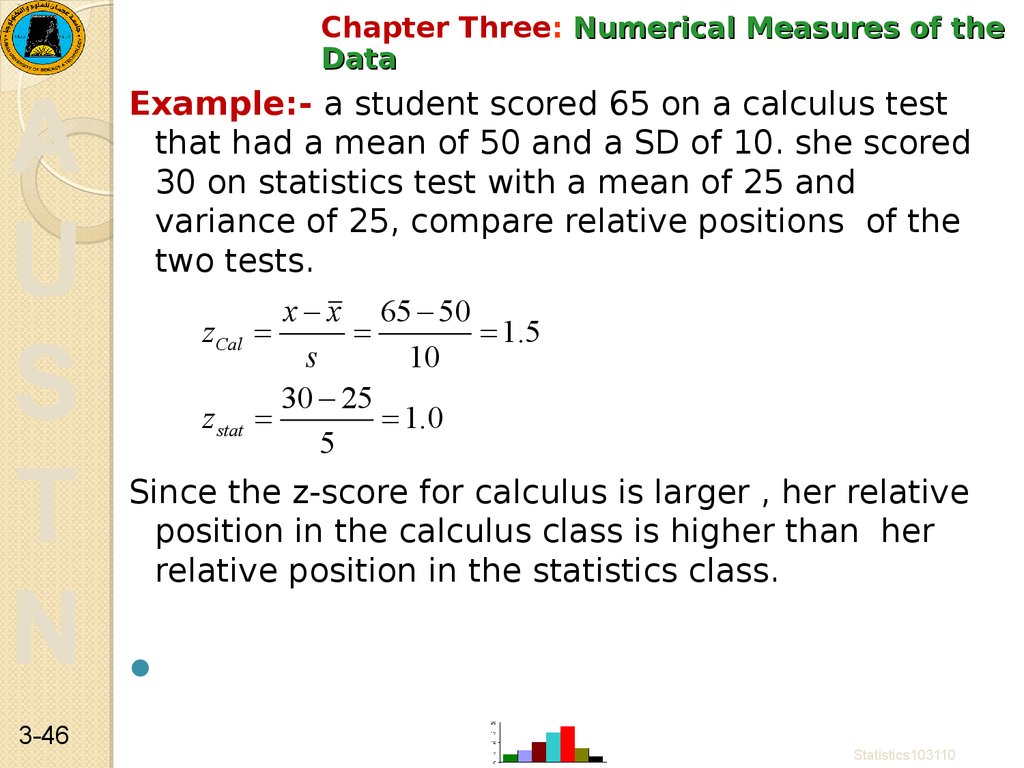
3-46
Example:- a student scored 65 on a calculus test
that had a mean of 50 and a SD of 10. she scored
30 on statistics test with a mean of 25 and
variance of 25, compare relative positions of the
two tests.
zCal
z stat
x x 65 50
1 .5
s
10
30 25
1 .0
5
Since the z-score for calculus is larger , her relative
position in the calculus class is higher than her
relative position in the statistics class.
Statistics103110

47. Chapter Three: Numerical Measures of the Data

A
U
S
T
N
3-47
2. Quartiles
Quartiles divide the data set into 4 groups.
Quartiles are denoted by Q1, Q2, and Q3.
The median is the same as Q2.
Finding the Quartiles
th
Procedure: Let Qk be the k quartile and n the sample
size.
Step 1: Arrange the data in order.
Step 2: Compute c = ({n+1} k)/4.
)/4
Step 3: If c is not a whole number, round off to whole number. use
the value halfway between xc and xc .1
Step 4: If c is a whole number then the value of xcis the position
value of the required percentile.
Statistics103110

48. Chapter Three: Numerical Measures of the Data

A
U
S
T
N
3-48
Example:
For the following data set: 2, 3, 5, 6, 8, 10, 12
Find Q1 and Q3
n = 7, so for Q1 we have c = ((7+1) 1)/4 = 2.
Hence the value of Q1 is the 2nd value.
Thus Q1 for the data set is
3.
for Q3 we have c = ((7+1) 3)/4 = 6.
Hence the value of Q3 is the 6th value.
Thus Q3 for the data set is
10.
Statistics103110

49. Chapter Three: Numerical Measures of the Data

A
U
S
T
N
3-49
Example: Find Q1 and Q3 for the following data set:
2, 3, 5, 6, 8, 10, 12, 15, 18.
Note: the data set is already ordered.
n = 9, so for Q1 we have c = ((9+1) 1)/4 = 2.5.
Hence the value of Q1 is the halfway between the 2nd
value and 3rd value.
3 5
Q1
2
4
for Q3 we have c = ((9+1) 3)/4 = 7.5.
Hence the value of Q3 is the halfway between the 7th
value and 8th value
12 15
Q3
13.5
2
Statistics103110

50. Chapter Three: Numerical Measures of the Data

A
U
S
T
N
3-50
Example:
For the following data set: 2, 3, 5, 6, 8, 10, 12
Find Q1 and Q3
The median for the above data is 6
The median for the lower group of data which is less than
median is 3
So the value of Q1 is the 2nd value which means that Q1 =3.
The median for the upper group of data which is grater
than median is 10
So the value of Q3 is the 6th value which means that Q3
=10.
Statistics103110

51. Chapter Three: Numerical Measures of the Data

A
U
S
T
N
3-51
The Q1 can be obtained graphically using the Ogive
locate the point, which
represent the value
obtained from
(division n by 4; 34/4 =
8.5)
And draw a horizontal
line until it intersects the
Ogive then draw a
vertical line until it
intersects the X-axis.
The intersection
represent the Q1
Value of Q1
Statistics103110

52. Chapter Three: Numerical Measures of the Data

A
U
S
T
N
3-52
The Q3 can be obtained graphically using the Ogive
locate the point, which
represent the value
(of 3n by 4; (3*34)/4 =
25.5)
And draw a horizontal
line until it intersects the
Ogive then draw a
vertical line until it
intersects the X-axis.
The intersection
represent the value of
Q3
Q3
Statistics103110

53. Chapter Three: Numerical Measures of the Data

A
U
S
T
N
3-53
The Interquartile Range (IQR)
The Interquartile Range, IQR = Q3 – Q1.
the  Interquartile Range  (IQR), also called
the midspread , middle fifty or inner
50% data range, is a measure
of statistical dispersion (variation), being
equal to the difference between the third
and first quartiles.
Statistics103110

54. Chapter Three: Numerical Measures of the Data

A
U
S
T
N
3-54
Outliers
An outlier is an extremely high or an extremely low data
value when compared with the rest of the data values .
To determine whether a data value can be
considered as an outlier:
Step 1: Compute Q1 and Q3.
Step 2: Find the IQR = Q3 – Q1.
Step 3: Compute (1.5)(IQR).
Step 4: Compute Q1 – (1.5)(IQR) and
Q3 + (1.5)(IQR).
they are called lower fence and upper fence
Step 5: Compare the data value (say X) with
lower and upper fences
If X < lower fence or if X > upper fence ,
then X is considered as an outlier.
Statistics103110

55. Example

Chapter Three: Numerical Measures of
the Data
A
U
S
T
N
3-55
Example
Given the data set 5, 6, 12, 13, 15, 18, 22, 50,
can the value of 50 be considered as an
outlier?
Q1 = 9, Q3 = 20, IQR = 11. Verify.
Verify
(1.5)(IQR) = (1.5)(11) = 16.5.
9 – 16.5 = – 7.5 and 20 + 16.5 = 36.5.
The value of 50 is outside the range (– 7.5 to
36.5), hence 50 is an outlier.
Statistics103110

56. Chapter Three: Numerical Measures of the Data

A
U
S
T
N
3-56
Measure of Dispersion tells us about the variation of the
data set.
Skewness tells us about the direction of variation of the
data set.
Definition:
Skewness is a measure of symmetry, or more precisely, the
lack of symmetry.
Coefficient of Skewness
Unitless number that measures the degree and direction of
symmetry of a distribution
There are several ways of measuring Skewness:
Pearson’s coefficient of Skewness
 
3 mean median
sk 2
s
Statistics103110

57. Chapter Three: Numerical Measures of the Data

A
U
S
T
N
The Empirical (Normal) Rule
For any bell shaped distribution:
Approximately 68% of the data values will fall
within one standard deviation of the mean.
Approximately 95% will fall within two standard
deviations of the mean.
Approximately 99.7% will fall within three
standard deviations of the mean.
= 95%
3-57
Statistics103110

58. The Empirical (Normal) Rule

Chapter Three: Numerical Measures of
the Data
A
U
S
T
N
3-58
The Empirical (Normal) Rule
= 95%
Statistics103110

59. Chapter Three: Numerical Measures of the Data

A
U
S
T
N
3-59
What is a Box Plot
To construct a box plot, first obtain the 5
number summary
{
Min,
Q1 ,
M,
Q3,
Max
}
The box-plot is a graphical representation of data
When the data set contains a small number of
values, a box plot is used to graphically represent
the data set. These plots involve five values: the
minimum value (the smallest value which is not
an outlier), the first quartile, the median, the
third quartile, and the maximum value (the
largest value which is not an outlier).
Statistics103110

60. Chapter Three: Numerical Measures of the Data

The box plot is useful in analyzing
small data sets that do not lend
themselves easily to histograms.
Because of the small size of a box
plot, it is easy to display and
compare several box plots in a small
space.
A box plot is a good alternative or
complement to a histogram and is
usually better for showing several
simultaneous comparisons.
3-60
Statistics103110

61. Chapter Three: Numerical Measures of the Data

How to use it:
Collect and arrange data.
Collect the data and
arrange it into an ordered set from lowest value to highest.
Calculate
Calculate
Calculate
Calculate
the
the
the
the
median. M = median= Q2
first quartile. (Q1)
third quartile. (Q3)
interquartile rage (IQR).
This
range is the difference between the first and third quartile
vales. (Q3 - Q1)
Obtain the maximum.
This is the largest data value
that is less than or equal to the third quartile plus 1.5 X IQR.
Q3 + [(Q3 - Q1) X 1.5]
.
3-61
Statistics103110

62. Chapter Three: Numerical Measures of the Data

Obtain the minimum.
This value will be the
smallest data value that is greater than or equal to the
first quartile minus 1.5 X IQR.
Q1 - [(Q3 - Q1) X 1.5]
Draw and label the axes of the graph.
The scale of the horizontal axis must be large enough to
encompass the greatest value of the data sets.
Draw the box plots.
Construct the box, insert median
points, and attach maximum and minimum. Identify outliers
(values outside the upper and lower fences) with asterisks.
The box plot can provide answers to the following
questions:
3-62
1.
Does the location differ between subgroups?
2.
Does the variation differ between subgroups?
3.
Are there any outliers?
Statistics103110

63. Chapter Three: Numerical Measures of the Data

A
U
S
T
N
3-63
Example 1:- Failure times of industrial machines (in hours)
32.56 42.02
65.52 66.54
5 # summary:
47.26 50.25 59.03 60.17 61.56 62.16
68.71 70.60 71.27 76.33 80.37 82.87
{ 32.56 , 59.03 , 63.29 , 70.60 , 82.87 }
62.84
63.29
63.52
The final product: A Simple Box-plot. Only quartile information is displayed.
A mathematical rule designates “outliers.” These are plotted using special symbols.
Statistics103110

64. Chapter Three: Numerical Measures of the Data

A
U
S
T
N
3-64
Statistics103110

65. Chapter Three: Numerical Measures of the Data

A
U
S
T
N
3-65
Chapter Three: Numerical Measures of the
Data
Now find the interquartile range (IQR). The interquartile range
is the difference between the upper quartile and the lower
quartile. In this case the IQR = 87 - 52 = 35. The IQR is a
very useful measurement. It is useful because it is less
influenced by extreme values, it limits the range to the
middle 50% of the values.
35 is the interquartile range
begin to draw Box-plot graph.
Statistics103110

66. Chapter Three: Numerical Measures of the Data

A
U
S
T
N
3-66
Example 2
Consider two datasets:
A1={0.22, -0.87, -2.39, -1.79, 0.37, -1.54, 1.28, -0.31, -0.74, 1.72,
0.38, -0.17, -0.62, -1.10, 0.30, 0.15, 2.30, 0.19, -0.50, -0.09}
A2={-5.13, -2.19, -2.43, -3.83, 0.50, -3.25, 4.32, 1.63, 5.18, -0.43,
7.11, 4.87, -3.10, -5.81, 3.76, 6.31, 2.58, 0.07, 5.76, 3.50}
Notice that both datasets are approximately balanced
around zero; evidently the mean in both cases is
"near" zero. However there is substantially more
variation in A2 which ranges approximately from -6 to
6 whereas A1 ranges approximately from -2½ to 2½.
Below find box plots. Notice the difference in scales:
since the box plot is displaying the full range of
variation, the y-range must be expanded.
Statistics103110

67. Chapter Three: Numerical Measures of the Data

A
U
S
T
N
3-67
Statistics103110

68. Chapter Three: Numerical Measures of the Data

A
U
S
T
N
3-68
Statistics103110

69.

Chapter Three: Numerical Measures of the
Data
A
U
S
T
N
3-69
Information Obtained from a Box Plot
1.
If the median is near the center of the box, the distribution is
approximately symmetric.
2.
If the median falls to the left of the center of the box, the
distribution is positively skewed.
3.
If the median falls to the right of the center of the box, the
distribution is negatively skewed
Similarly :
1.
If the lines are about the same length, the distribution is
approximately symmetric.
2.
If the right line is larger than the left line, the distribution is
positively skewed.
3.
If the left line is larger than the right line, the distribution is
negatively skewed.
Statistics103110