


 mathematics
Similar presentations:

")


Descriptive statistics. Elementary statistics. Larson. Farber. (Chapter 2)
1. Descriptive Statistics
Chapter2
Descriptive Statistics
Elementary Statistics
Larson
Farber
1
2. Frequency Distributions
Minutes Spent on the Phone102
71
103
105
109
124
104
116
97
99
108 86 103
112 118 87
85 122 87
107 67 78
105 99 101
82
95
100
125
92
Make a frequency distribution table with five classes.
Key values:
Minimum value =
Maximum value =
67
125
2
3. Frequency Distributions
Decide on the number of classes (For this problem use 5)Calculate the Class Width
(125 - 67) / 5 = 11.6 Round up to 12
Determine Class Limits
Mark a tally in appropriate class for each data value
Class Limits
Tally
f
67
78
3
79
90
5
91
102
8
103
114
9
115
126
5
Do all lower class limits first.
f =30
3
4.
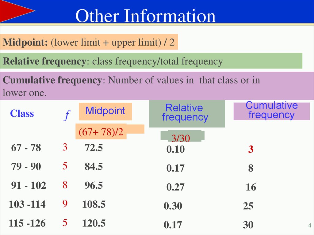
Other InformationMidpoint: (lower limit + upper limit) / 2
Relative frequency: class frequency/total frequency
Cumulative frequency: Number of values in that class or in
lower one.
Cumulative
Relative
Midpoint
Class
frequency
f
frequency
(67+ 78)/2
3/30
3
67 - 78
72.5
0.10
3
79 - 90
5
84.5
0.17
8
91 - 102
8
96.5
0.27
16
103 -114
9
108.5
0.30
25
115 -126
5
120.5
0.17
30
4
5. Frequency Histogram
Classf
Boundaries
67 - 78
3
66.5 - 78.5
79 - 90
5
78.5 - 90.5
91 - 102
8
90.5 - 102.5
103 -114
9 102.5 -114.5
115 -126
5 115.5 -126.5
Time on Phone
9
9
8
8
7
6
5
5
f
5
4
3
3
2
1
0
66.5
78.5
90.5
102.5
114.5
126.5
minutes
5
6. Frequency Polygon
Classf
67 - 78
3
79 - 90
5
Time on Phone
f
9
9
91 - 102
103 -114
115 -126
8
9
5
8
8
7
6
5
5
5
4
3
3
2
1
0
72.5
84.5
96.5
108.5
120.5
minutes
Mark the midpoint at the top of each bar. Connect consecutive
midpoints. Extend the frequency polygon to the axis.
6
7. Relative Frequency Histogram
Time on Phone.30
.30
.27
.20
.17
.17
.10
.10
0
66.5
78.5
90.5
102.5 114.5 126.5
minutes
Relative frequency on vertical scale
7
8. Ogive
Cumulative FrequencyAn ogive reports the number of values in the data set that
are less than or equal to the given value, x.
Minutes on Phone
30
30
25
20
16
10
8
3
0
0
66.5
78.5
90.5
102.5
114.5
126.5
minutes
8
9. Stem-and-Leaf Plot
Lowest value is 67 and highest value is 125, so liststems from 6 to 12.
102
Stem
6 |
7 |
8 |
9 |
10|
11|
12|
124
108
86
103
82
Leaf
6
2
2
8
4
3
9
10. Stem-and-Leaf Plot
Key: 6 | 7 means 676 |7
7 |1 8
8 |2 5 6 7 7
9 |2 5 7 9 9
10 |0 1 2 3 3 4 5 5 7 8 9
11 |2 6 8
12 |2 4 5
10
11. Stem-and-Leaf with two lines per stem
Key: 6 | 7 means 671st line digits 0 1 2 3 4
2nd line digits 5 6 7 8 9
1st line digits 0 1 2 3 4
2nd line digits 5 6 7 8 9
6|7
7|1
7|8
8|2
8|5677
9|2
9|5799
10 | 0 1 2 3 3 4
10 | 5 5 7 8 9
11 | 2
11 | 6 8
12 |2 4
12 | 5
11
12. Dotplot
Phone66
76
86
96
106
116
126
minutes
12
13. Pie Chart
Used to describe parts of a wholeCentral Angle for each segment
number in category
o
360
total number
The 1995 NASA budget (billions of $)
divided among 3 categories.
Billions of $
Human Space Flight
5.7
Technology
5.9
Mission Support
2.7
Construct a pie chart for the data.
13
14. Pie Chart
Human Space FlightTechnology
Mission Support
Billions of $Angle(deg.)
5.7
143
5.9
149
2.7
68
14.3
Total
5.7/14.3*360o = 143o
NASA Budget
5.9/14.3*360o = 149o
(Billions of $)
Mis s ion
Support
19%
Technology
41%
Hum an
Space Flight
40%
14
15. Measures of Central Tendency
Mean: The sum of all data values divided by thenumber of values
For a sample:
x
x
x
N
n
Median: The point at which an equal number of
values fall above and fall below
For a population:
Mode: The value with the highest frequency
15
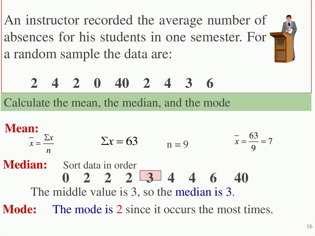
16.
An instructor recorded the average number ofabsences for his students in one semester. For
a random sample the data are:
2 4 2 0 40 2 4
3 6
Calculate the mean, the median, and the mode
Mean:
x
x
n
Median:
x 63
n=9
x
63
7
9
Sort data in order
0 2 2
2 3 4 4 6
40
The middle value is 3, so the median is 3.
Mode: The mode is 2 since it occurs the most times.
16
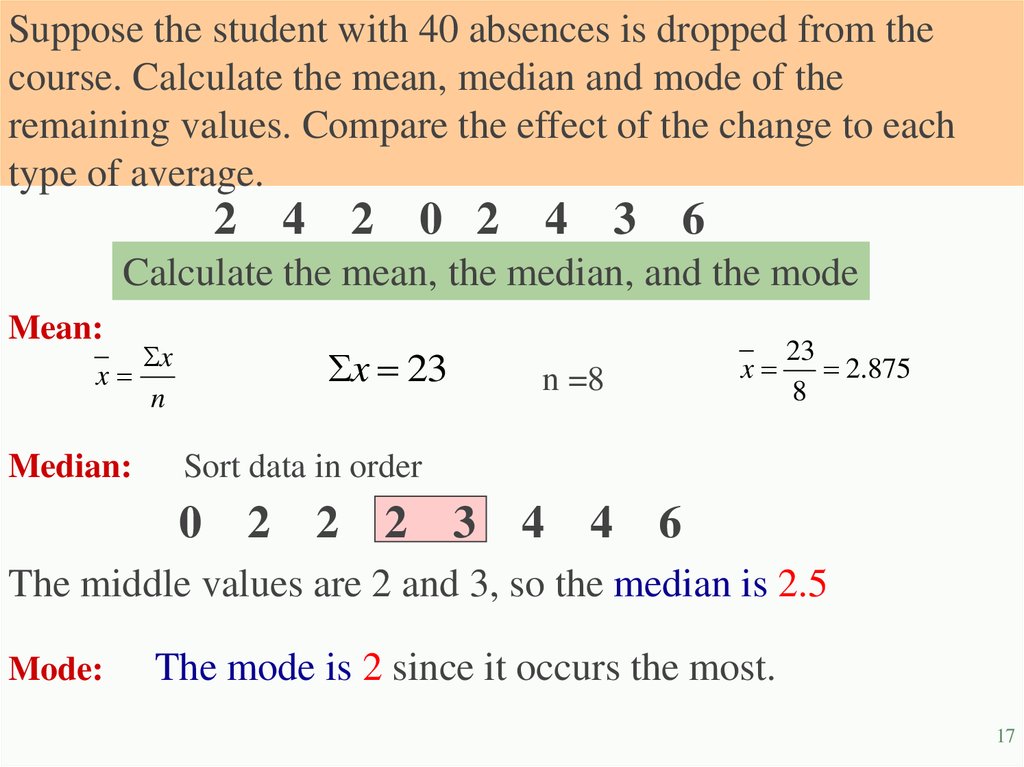
17.
Suppose the student with 40 absences is dropped from thecourse. Calculate the mean, median and mode of the
remaining values. Compare the effect of the change to each
type of average.
2 4 2 0 2 4 3 6
Calculate the mean, the median, and the mode
Mean:
x
x
n
Median:
x 23
n =8
x
23
2.875
8
Sort data in order
0 2 2 2 3 4 4 6
The middle values are 2 and 3, so the median is 2.5
Mode:
The mode is 2 since it occurs the most.
17
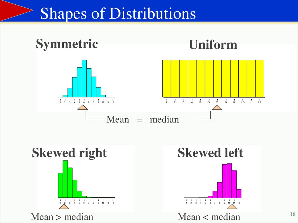
18.
Shapes of DistributionsSymmetric
1
2
3
4
5
6
7
8
9
Uniform
10
11
12
1
2
3
4
5
6
7
8
9
10
11
12
Mean = median
Skewed right
1
2
3
4
5
6
7
8
Mean > median
9
10
11
Skewed left
12
1
2
3
4
5
6
7
8
9
10
11
12
Mean < median
18
19. Descriptive Statistics
Closing prices for two stocks were recorded on ten successiveFridays. Calculate the mean, median and mode for each.
Stock A
Mean = 61.5
Median =62
Mode= 67
56
56
57
58
61
63
63
67
67
67
33 Stock B
42
48
52
57
67
67
77 Mean = 61.5
82 Median =62
90 Mode= 67
19
20. Measures of Variation
Range = Maximum value - Minimum valueRange for A = 67 - 56 = $11
Range for B = 90 - 33 = $57
The range only uses 2 numbers from a data set.
The deviation for each value x is the difference
between the value of x and the mean of the data set.
In a population, the deviation for each value x is:x
In a sample, the deviation for each value x is:
-
x x
20
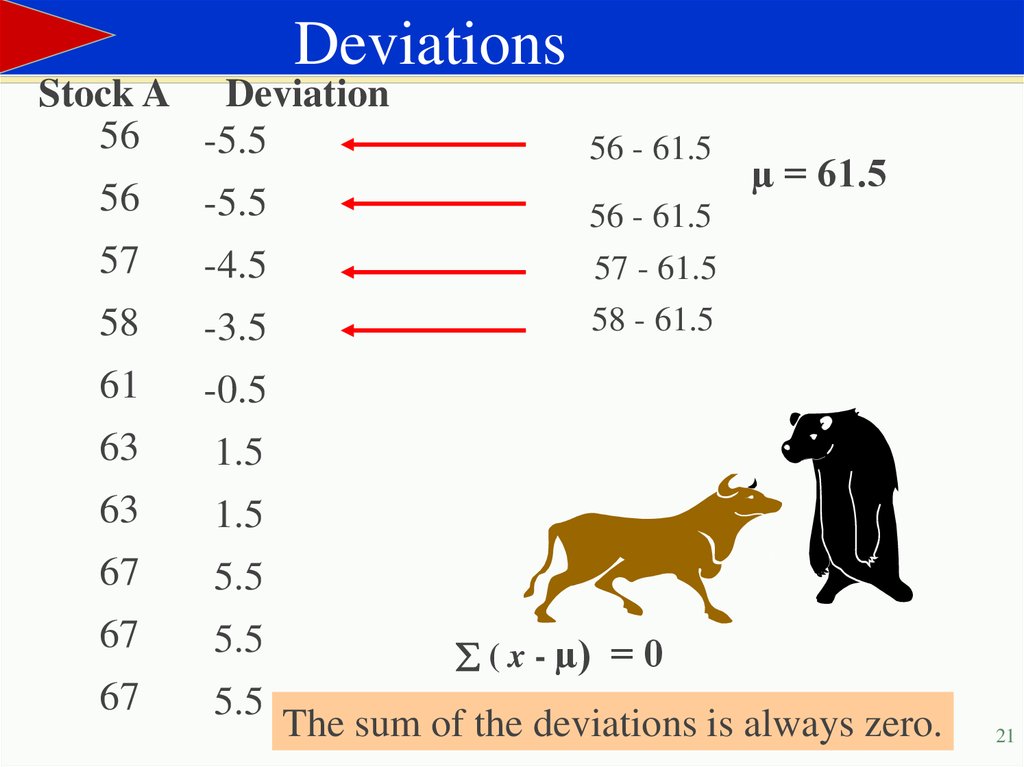
21.
DeviationsStock A Deviation
56
-5.5
56
-5.5
57
-4.5
58
-3.5
61
-0.5
63
1.5
63
1.5
67
5.5
67
5.5
67
5.5
56 - 61.5
µ = 61.5
56 - 61.5
57 - 61.5
58 - 61.5
( x - µ) = 0
The sum of the deviations is always zero.
21
22. Population Variance
xPopulation Variance
Population Variance: The sum of the squares of the
deviations, divided by N.
x ( x )2
Stock A
56
56
57
58
61
63
63
67
67
67
-5.5
-5.5
-4.5
-3.5
-0.5
1.5
1.5
5.5
5.5
5.5
( x ) 2
N
30.25
2
30.25
20.25
12.25
188.50
2
0.25
2.25
10
2.25
30.25
30.25
30.25
Sum of squares
188.50
18.85
22
23. Population Standard Deviation
Population Standard Deviation The square root ofthe population variance.
2
18.85 4.34
The population standard deviation is $4.34
23
24. Sample Standard Deviation
To calculate a sample variance divide the sum ofsquares by n-1.
2
(
x
x
)
188.50
s2
20.94
s2
9
n 1
The sample standard deviation, s is found by taking the
square root of the sample variance.
s s
2
s 20.94 4.58
Calculate the measures of variation for Stock B
24
25. Summary
Range = Maximum value - Minimum valuePopulation Variance
2
( x )
N
2
( x x )
n 1
2
Population Standard Deviation
Sample Variance
s
2
Sample Standard Deviation
s s
2
2
25
26. Empiricl Rule 68- 95- 99.7% rule
Data with symmetric bell-shaped distribution has thefollowing characteristics.
13.5%
13.5%
68%
2.35%
4
3
2.35%
2
1
0
1
2
3
4
About 68% of the data lies within 1 standard deviation of the mean
About 95% of the data lies within 2 standard deviations of the mean
About 99.7% of the data lies within 3 standard deviations of the mean
26
27. Using the Empirical Rule
The mean value of homes on a street is $125 thousand with a standarddeviation of $5 thousand. The data set has a bell shaped distribution.
Estimate the percent of homes between $120 and $135 thousand
68%
68%
105
110
115
120
13.5%
68%
125
130
135
140
145
$120 is 1 standard deviation below the mean and $135 thousand is 2
standard deviation above the mean. 68% + 13.5% = 81.5%
So, 81.5% of the homes have a value between $120 and $135 thousand .
27
28. Chebychev’s Theorem
For any distribution regardless of shape the portion of datalying within k standard deviations (k >1) of the mean is at
least 1 - 1/k2.
=6
=3.84
1
2
3
4
5
6
7
8
9
10
11
12
For k = 2, at least 1-1/4 = 3/4 or 75% of the data lies within 2
standard deviation of the mean.
For k = 3, at least 1-1/9 = 8/9= 88.9% of the data lies within 3
standard deviation of the mean.
28
29. Chebychev’s Theorem
The mean time in a women’s 400-meter dash is 52.4seconds with a standard deviation of 2.2 sec. Apply
Chebychev’s theorem for k = 2.
Mark a number line in
standard deviation units.
2 standard deviations
45.8
48
50.2
52.4
54.6
56.8
59
At least 75% of the women’s 400- meter dash times
will fall between 48 and 56.8 seconds.
29
30. Grouped Data
To approximate the mean of data in a frequency distribution,( x f )
treat each value as if it occurs at the midpoint
x
of its class. x = Class midpoint.
n
Class
67- 78
79- 90
91- 102
103-114
115-126
f
3
5
8
9
5
30
Midpoint (x)
72.5
84.5
96.5
108.5
120.5
x f
217.
5
422.
5
722.0
976.5
602.5
2991
2991
x
99.7
30
30
31. Grouped Data
To approximate the standard deviation of datain a frequency distribution,
use x = class midpoint.
s
( x x ) f
n 1
2
x 99.7
Class
67- 78
79- 90
91- 102
103-114
115-126
f
3
5
8
9
5
30
( x x )2
Midpoint
72.5
739.84
84.5
231.04
96.5
10.24
108.5
77.44
120.5
432.64
( x x )2 * f
2219.52
1155.20
81.92
696.96
2163.2
6316.8
6316.8
s
217.8207 14.76
29
31
32.
Quartiles3 quartiles Q1, Q2 and Q3 divide the data into 4 equal parts.
Q2 is the same as the median.
Q1 is the median of the data below Q2
Q3 is the median of the data above Q2
You are managing a store. The average sale for each
of 27 randomly selected days in the last year is
given. Find Q1, Q2 and Q3..
28 43 48 51 43 30 55 44 48 33 45 37 37 42
27 47 42 23 46 39 20 45 38 19 17 35 45
32
33.
QuartilesThe data in ranked order (n = 27) are:
17 19 20 23 27 28 30 33 35 37 37 38 39 42 42
43 43 44 45 45 45 46 47 48 48 51 55 .
Median rank (27 +1)/2 = 14. The median = Q2 = 42.
There are 13 values below the median.
Q1 rank= 7. Q1 is 30.
Q3 is rank 7 counting from the last value. Q3 is 45.
The Interquartile Range is Q3 - Q1 = 45 - 30 = 15
33
34. Box and Whisker Plot
A box and whisker plot uses 5 key values to describe a set of data.Q1, Q2 and Q3, the minimum value and the maximum value.
Q1
Q2 = the median
Q3
Minimum value
Maximum value
30
42
45
17
55
30
42
45
17
15
55
25
35
45
55
Interquartile Range
34
35. Percentiles
Percentiles divide the data into 100 parts. There are99 percentiles: P1, P2, P3…P99 .
P50 = Q2 = the median
P25 = Q1
P75 = Q3
A 63nd percentile score indicates that score is
greater than or equal to 63% of the scores and less
than or equal to 37% of the scores.
35
36. Percentiles
3030
25
20
16
10
8
3
0
0
66.5
78.5
90.5
102.5
114.5
126.5
Cumulative distributions can be used to find percentiles.
114.5 falls on or above 25 of the 30 values.
25/30 = 83.33.
So you can approximate 114 = P83 .
36