Similar presentations:
Genome assembly with SPAdes
1.
Genome assembly withSPAdes
Center for Algorithmic Biotechnology
SPbU
2.
Introduction3.
Why to assemble?4.
Why to assemble?● Sequencing data
○ Billions of short reads
○ Sequencing errors
○ Contaminants
5.
Why to assemble?● Sequencing data
○ Billions of short reads
○ Sequencing errors
○ Contaminants
● Assembly
✓
✓
✓
×
Corrects sequencing errors
Much longer sequences
Each genomic region is presented only once
May introduce errors
6.
Assembly basics7.
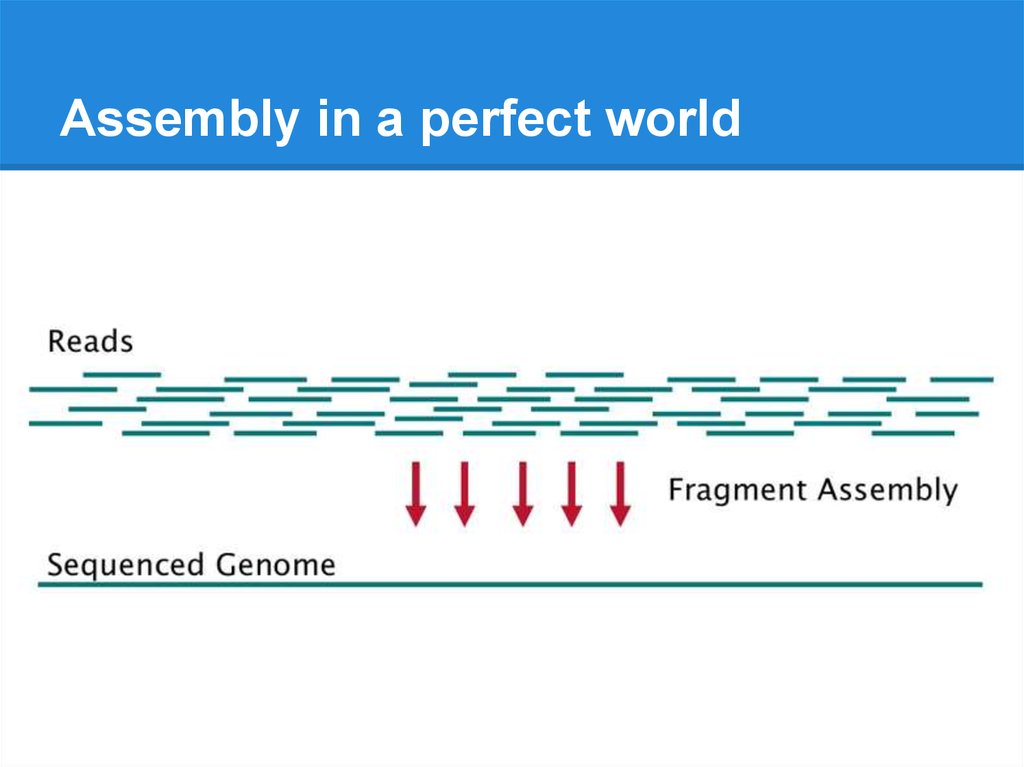
Assembly in a perfect world8.
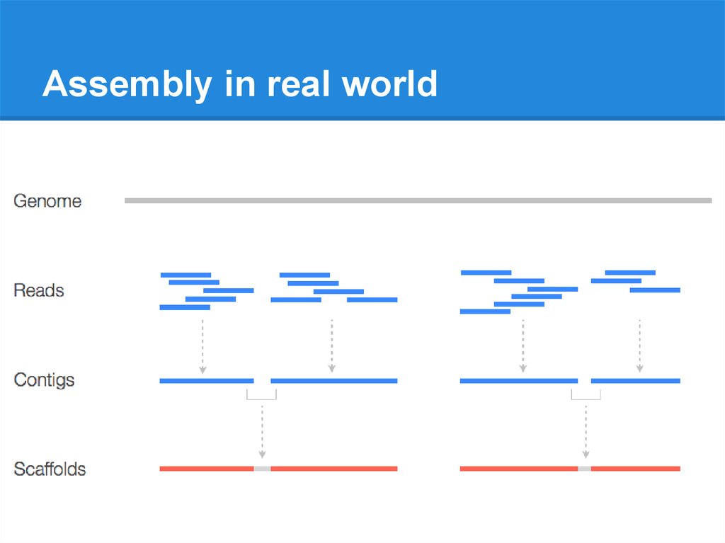
Assembly in real world9.
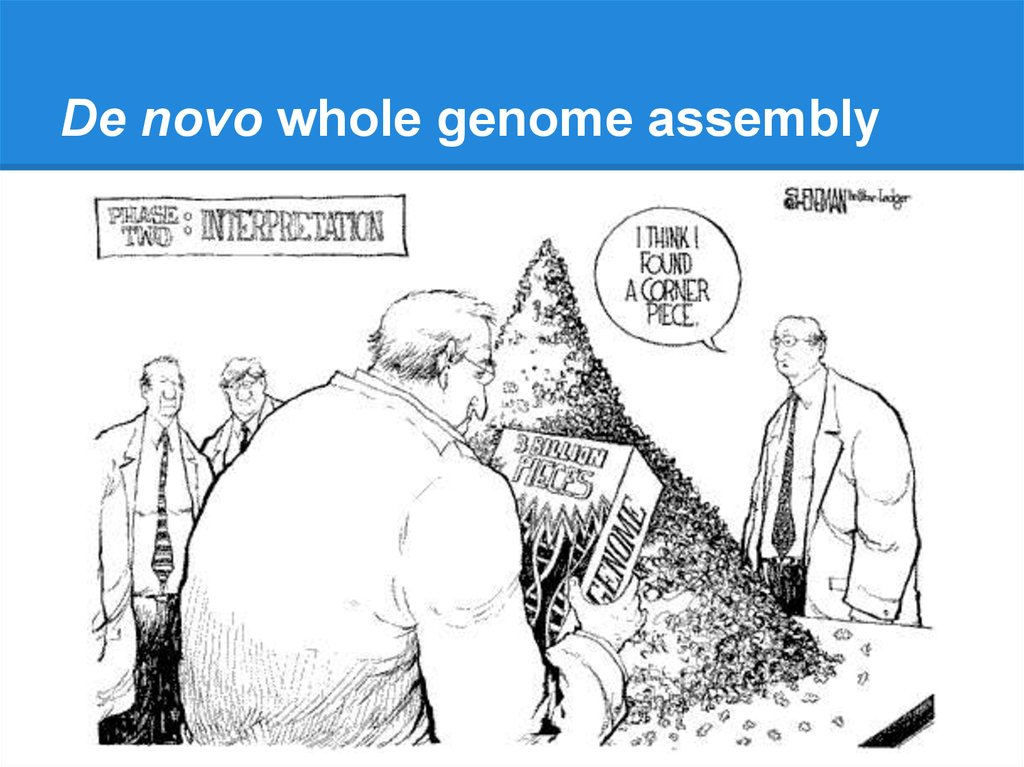
De novo whole genome assembly10.
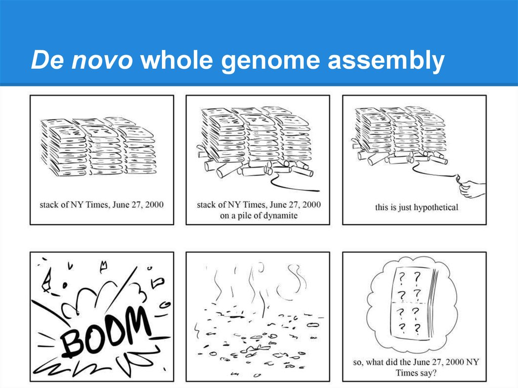
De novo whole genome assembly11.
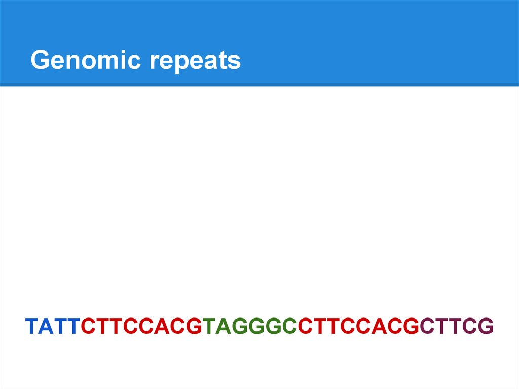
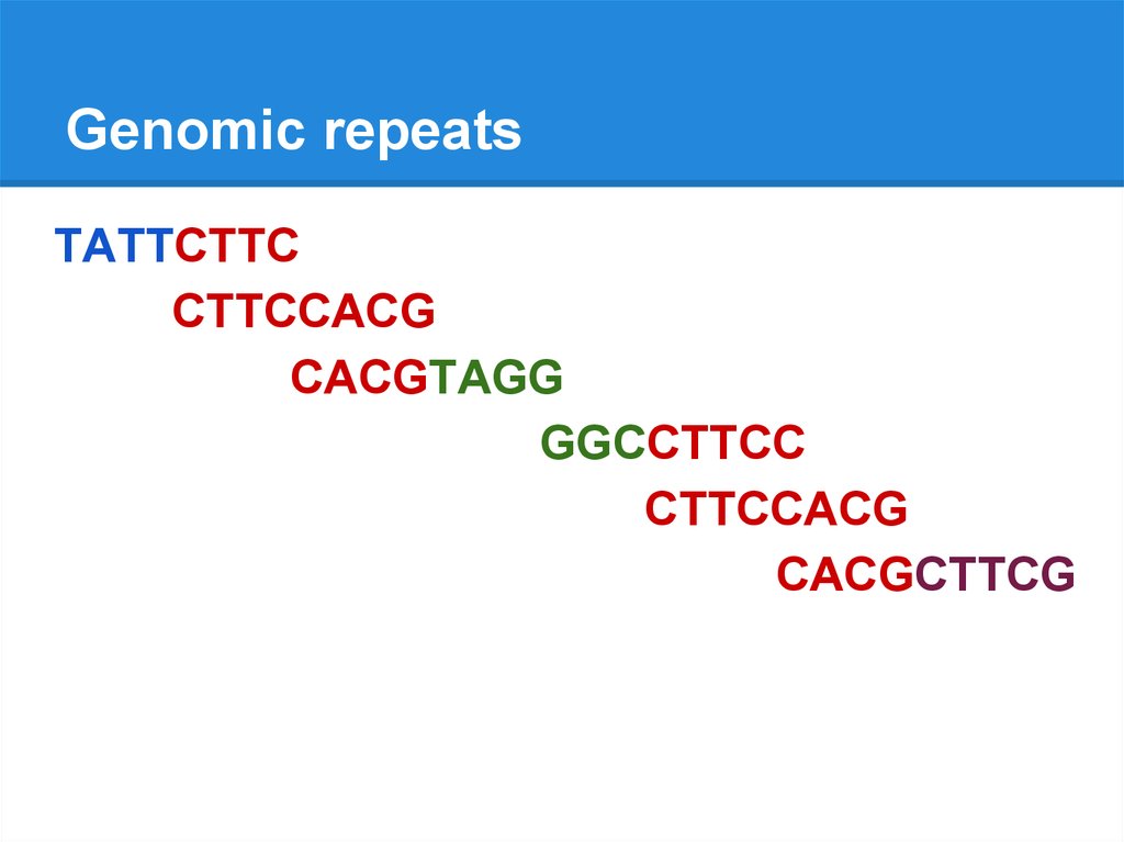
Genomic repeatsTATTCTTCCACGTAGGGCCTTCCACGCTTCG
12.
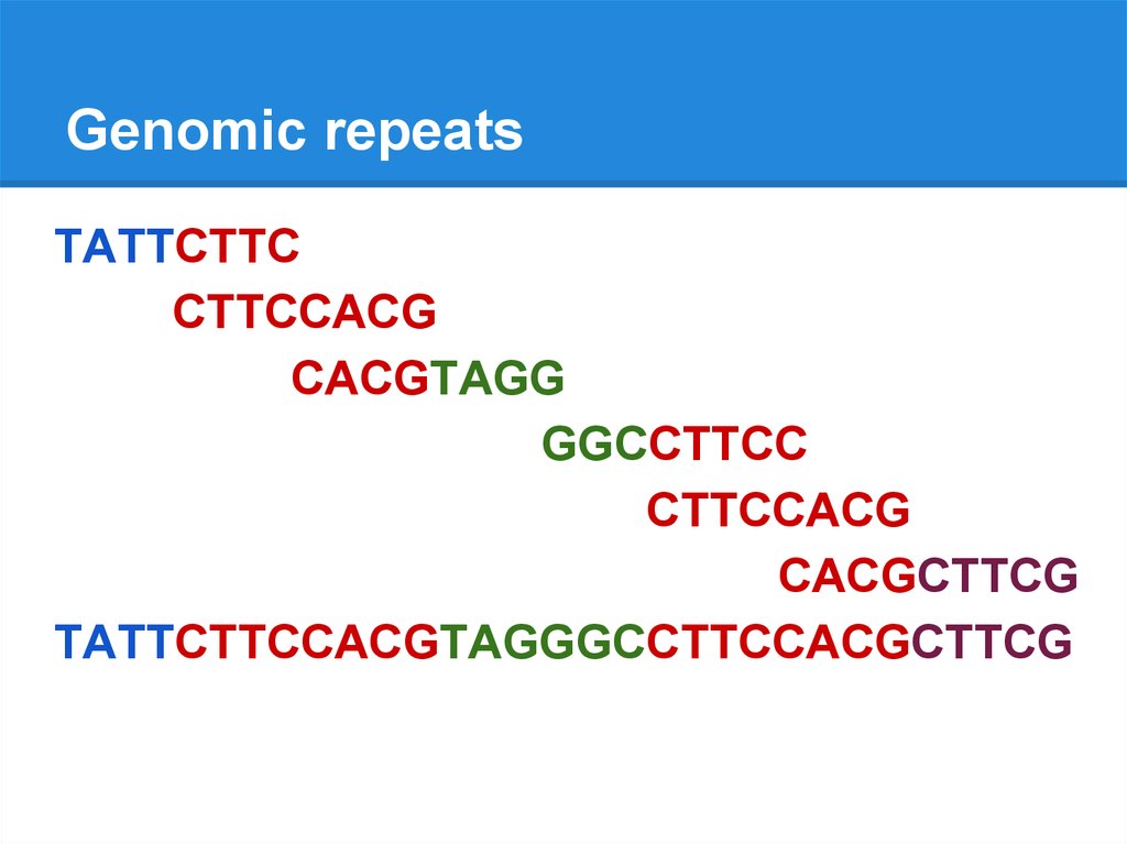
Genomic repeatsTATTCTTC
CTTCCACG
CACGTAGG
GGCCTTCC
CTTCCACG
CACGCTTCG
TATTCTTCCACGTAGGGCCTTCCACGCTTCG
13.
Genomic repeatsTATTCTTC
CTTCCACG
CACGTAGG
GGCCTTCC
CTTCCACG
CACGCTTCG
14.
Genomic repeatsTATTCTTCCACGTAGG
GGCCTTCCACGCTTCG
TATTCTTCCACGCTTCG
GGCCTTCCACGTAGG
15.
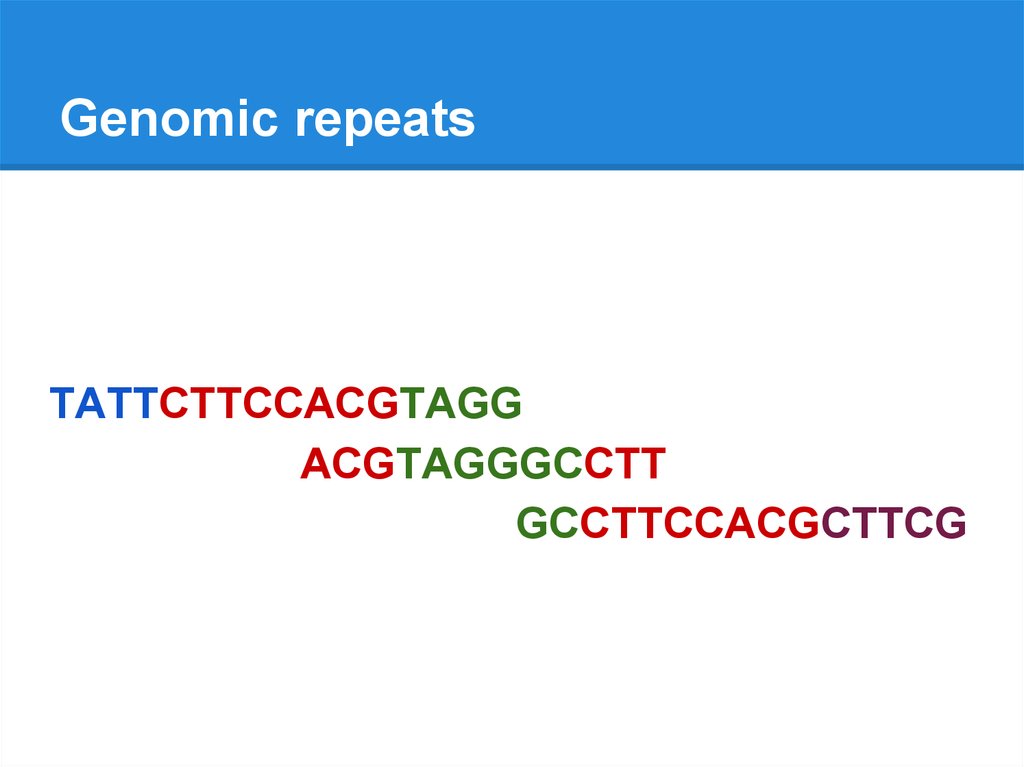
Genomic repeatsTATTCTTCCACGTAGG
ACGTAGGGCCTT
GCCTTCCACGCTTCG
TATTCTTCCACGTAGGGCCTTCCACGCTTCG
16.
Genomic repeatsTATTCTTCCACGTAGG
ACGTAGGGCCTT
GCCTTCCACGCTTCG
17.
SPAdes assembler18.
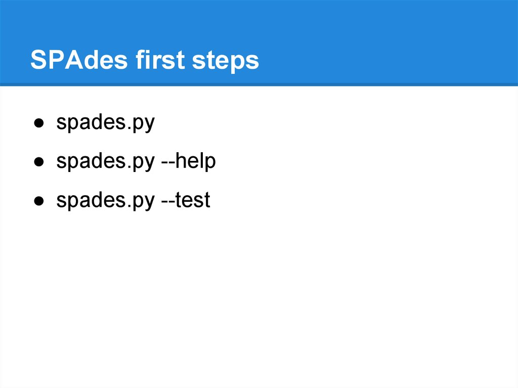
SPAdes first steps● spades.py
19.
SPAdes first steps● spades.py
● spades.py --help
● spades.py --test
20.
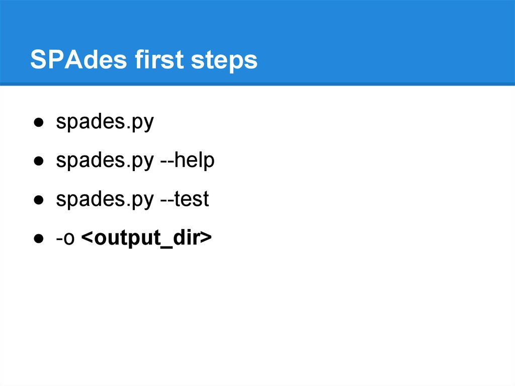
SPAdes first steps● spades.py
● spades.py --help
● spades.py --test
● -o <output_dir>
21.
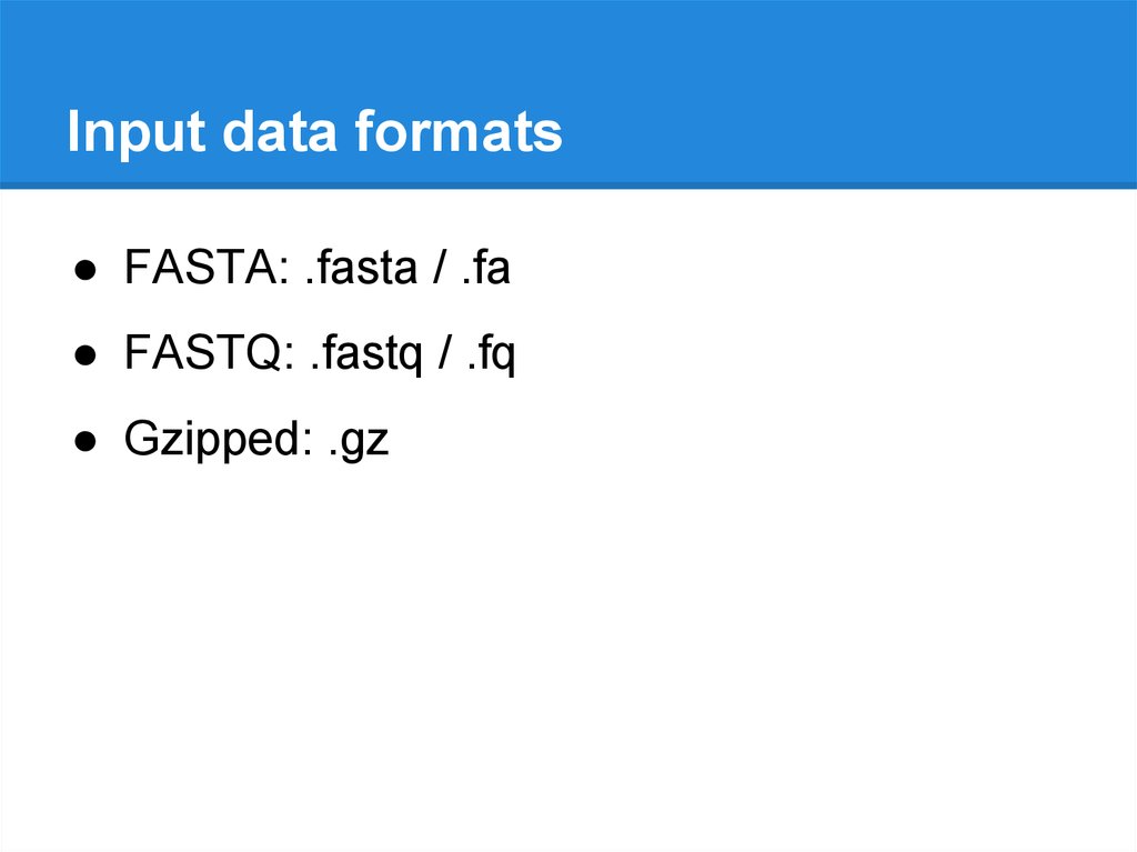
Input data formats● FASTA: .fasta / .fa
● FASTQ: .fastq / .fq
● Gzipped: .gz
22.
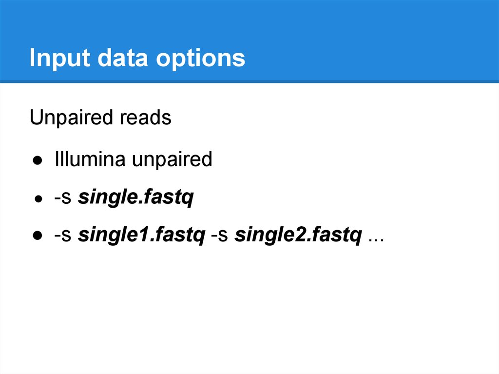
Input data optionsUnpaired reads
● Illumina unpaired
-s single.fastq
● -s single1.fastq -s single2.fastq ...
23.
Input data optionsPaired-end reads
● Interlaced pairs in one file
>left_read_id
ACGTGCAGG…
>right_read_id
GCTTCGAGG…
● Separate files
file1.fastq
>left_read_id
ACGTGCAGG…
file2.fastq
>right_read_id
GCTTCGAGG…
24.
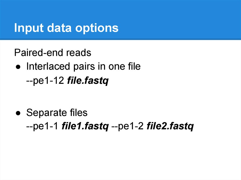
Input data optionsPaired-end reads
● Interlaced pairs in one file
--pe1-12 file.fastq
● Separate files
--pe1-1 file1.fastq --pe1-2 file2.fastq
25.
Input data optionsPaired-end reads
● Interlaced pairs in one file
--pe1-12 file.fastq
● Separate files
--pe1-1 file1.fastq --pe1-2 file2.fastq
--pe1-s unpaired.fastq
26.
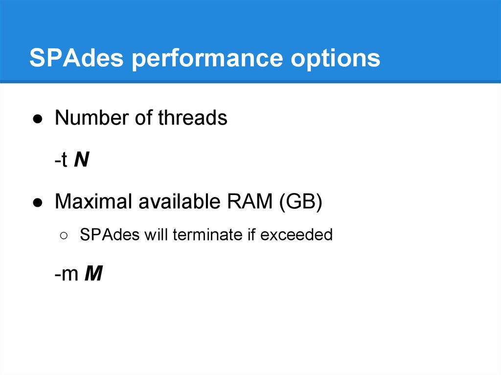
SPAdes performance options● Number of threads
-t N
● Maximal available RAM (GB)
○ SPAdes will terminate if exceeded
-m M
27.
Pipeline options● Run only assembler (input reads are already
corrected or quality-trimmed)
○ --only-assembler
28.
Input data optionsMate-pair reads
● Cannot be used separately
● Interlaced pairs in one file
--mp1-12 mp.fastq
● Separate files
--mp1-1 mp1.fastq --mp1-2 mp2.fastq
29.
Hybrid assembly options● PacBio CLR
○ --pacbio pb.fastq
● Oxford Nanopore reads
○ --nanopore nanopore_reads.fastq
30.
Restarting SPAdes● SPAdes / system crashed
○ --continue -o your_output_dir
31.
Genome assemblyevaluation with QUAST
Center for Algorithmic Biotechnology
SPbU
32.
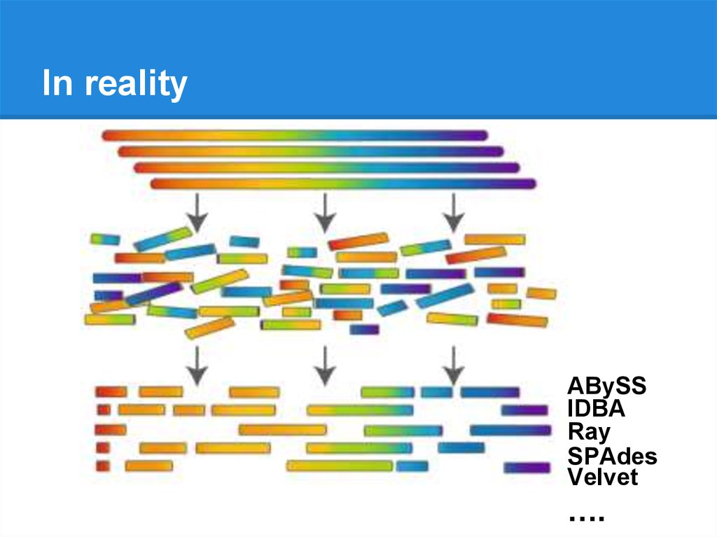
In realityABySS
IDBA
Ray
SPAdes
Velvet
….
33.
Which assembler to use?ABySS
ALLPATHS-LG
CLC
IDBA-UD
MaSuRCA
MIRA
Ray
SOAPdenovo
SPAdes
Velvet
and many more...
34.
Which assembler to use?● Different technologies (Illumina, 454,
IonTorrent, ...)
● Genome type and size (bacteria, insects,
mammals, plants, ...)
● Type of prepared libraries (single reads,
paired-end, mate-pairs, combinations)
● Type of data (multicell, metagenomic, singlecell)
35.
There is no best assembler36.
Which assembler to use?● Assemblathon 1 & 2
○ Simulated and real datasets
○ More than 30 teams competing
● Independent studies
○ Papers (GAGE, GAGE-B, GABenchToB)
○ Web-sites (nucleotid.es, …)
○ Surveys
● Genome assembly evaluation tools
○ QUAST
○ GAGE
37.
Assembly evaluation● Basic evaluation
○ No extra input
○ Very quick
● Reference-based evaluation
○ A lot of metrics
○ Very accurate
● De novo evaluation
○ Advanced analysis of de novo assemblies
38.
Basic statisticsOnly assemblies are needed (no additional input)
Very fast to compute
39.
Contig sizes● Number of contigs
40.
Contig sizes● Number of contigs
● Number of large contigs (i.e. > 1000 bp)
41.
Contig sizes● Number of contigs
● Number of large contigs (i.e. > 1000 bp)
● Largest contig length
42.
Contig sizes● Number of contigs
● Number of large contigs (i.e. > 1000 bp)
● Largest contig length
● Total assembly length
43.
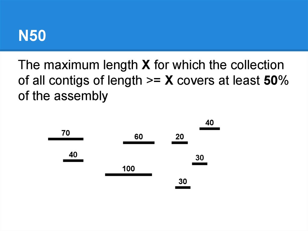
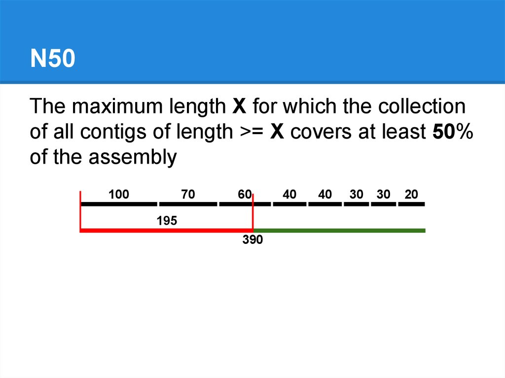
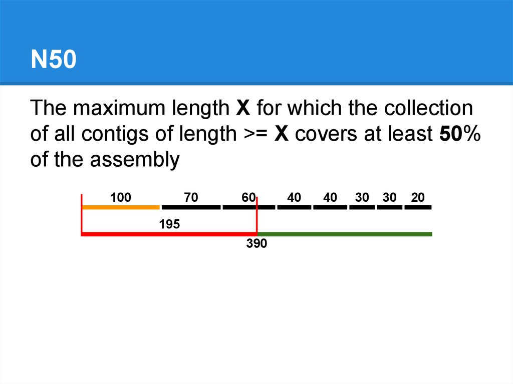
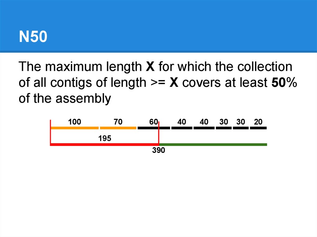
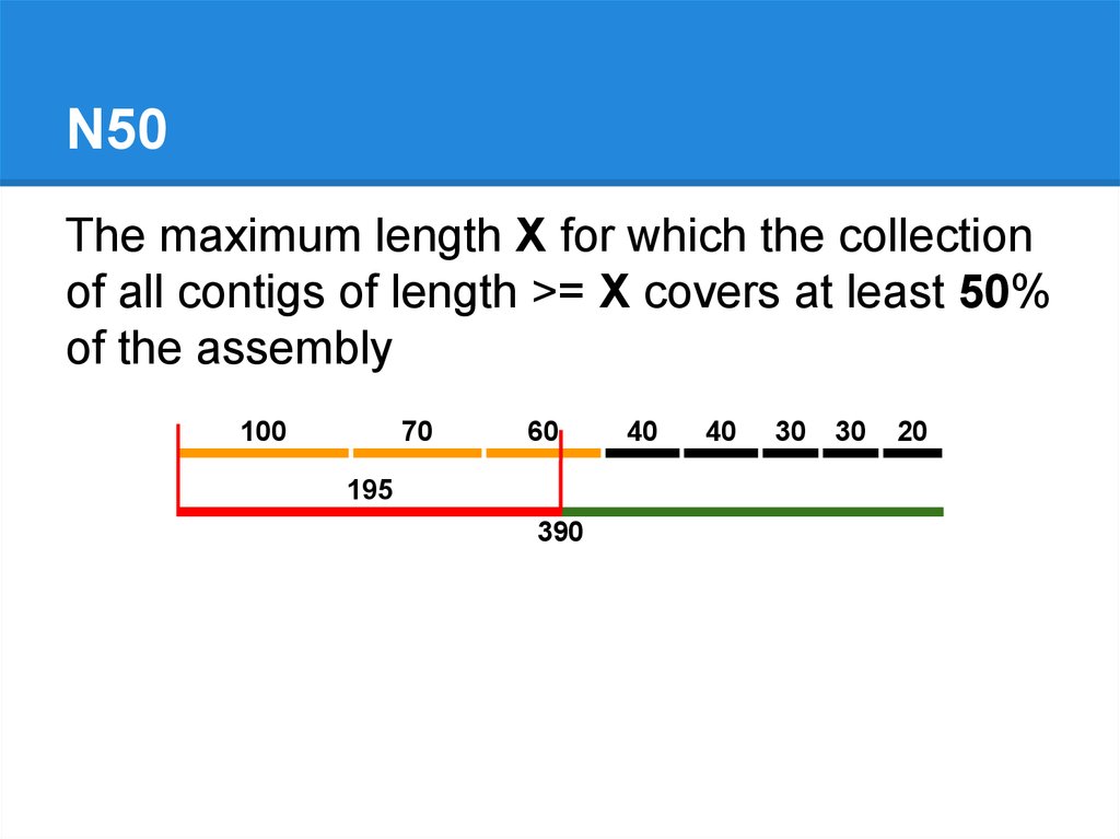
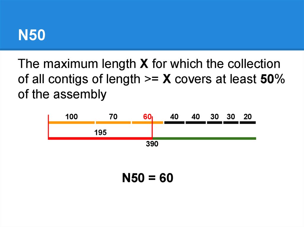
N50The maximum length X for which the collection
of all contigs of length >= X covers at least 50%
of the assembly
40
70
60
20
40
30
100
30
44.
N50The maximum length X for which the collection
of all contigs of length >= X covers at least 50%
of the assembly
100
70
60
40
40
30
30
20
45.
N50The maximum length X for which the collection
of all contigs of length >= X covers at least 50%
of the assembly
100
70
60
390
40
40
30
30
20
46.
N50The maximum length X for which the collection
of all contigs of length >= X covers at least 50%
of the assembly
100
70
60
195
390
40
40
30
30
20
47.
N50The maximum length X for which the collection
of all contigs of length >= X covers at least 50%
of the assembly
100
70
60
195
390
40
40
30
30
20
48.
N50The maximum length X for which the collection
of all contigs of length >= X covers at least 50%
of the assembly
100
70
60
195
390
40
40
30
30
20
49.
N50The maximum length X for which the collection
of all contigs of length >= X covers at least 50%
of the assembly
100
70
60
195
390
40
40
30
30
20
50.
N50The maximum length X for which the collection
of all contigs of length >= X covers at least 50%
of the assembly
100
70
60
40
195
390
N50 = 60
40
30
30
20
51.
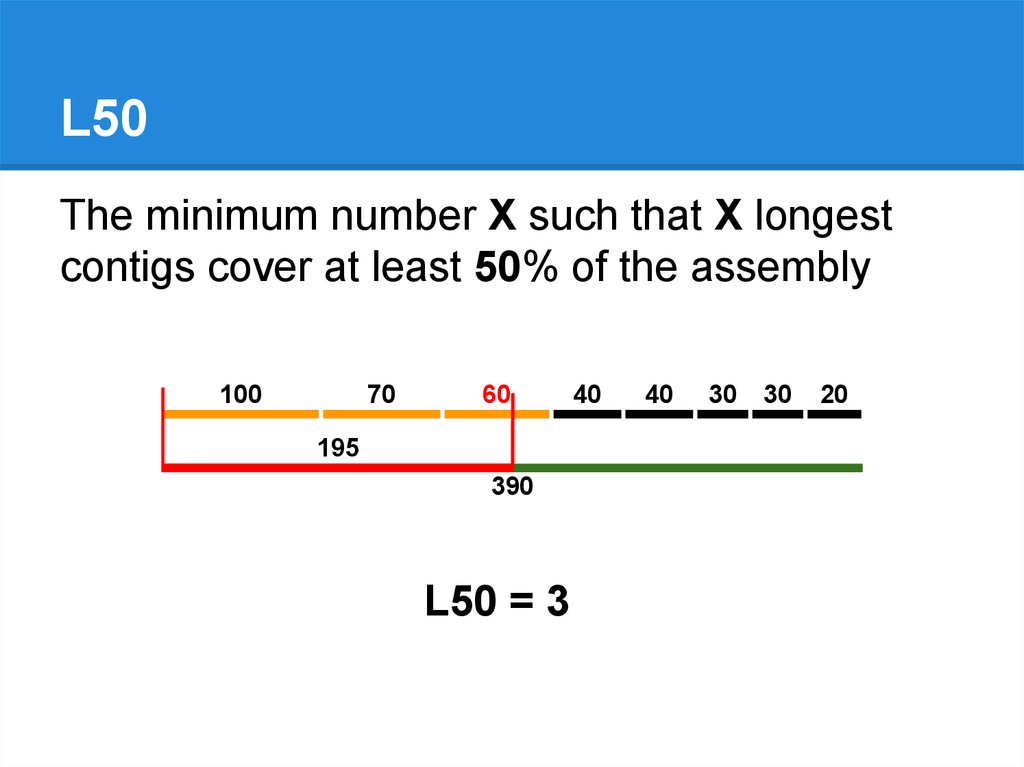
L50The minimum number X such that X longest
contigs cover at least 50% of the assembly
100
70
60
195
390
L50 = 3
40
40
30
30
20
52.
L50The minimum number X such that X longest
contigs cover at least 50% of the assembly
100
70
60
195
390
L50 = 3
40
40
30
30
20
53.
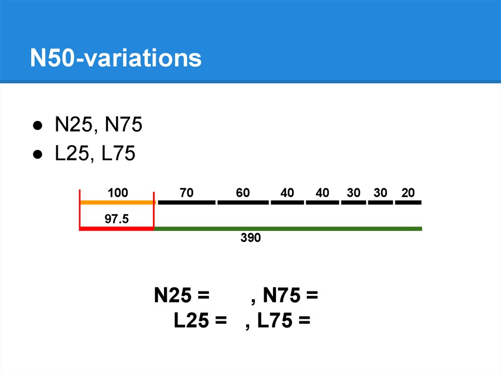
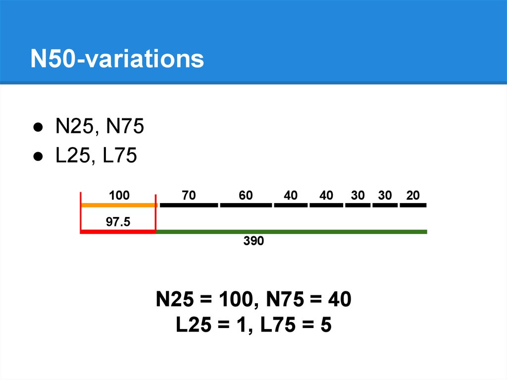
N50-variations● N25, N75
● L25, L75
100
70
60
40
40
30
97.5
390
N25 = 100, N75 = 40
L25 = 1, L75 = 5
30
20
54.
N50-variations● N25, N75
● L25, L75
100
70
60
40
40
30
97.5
390
N25 = 100, N75 = 40
L25 = 1, L75 = 5
30
20
55.
N50-variations● N25, N75
● L25, L50, L75
56.
N50-variations● N25, N75
● L25, L50, L75
● Nx, Lx
57.
Other● Number of N’s per 100 kbp
58.
Other● Number of N’s per 100 kbp
● GC %
59.
Other● Number of N’s per 100 kbp
● GC %
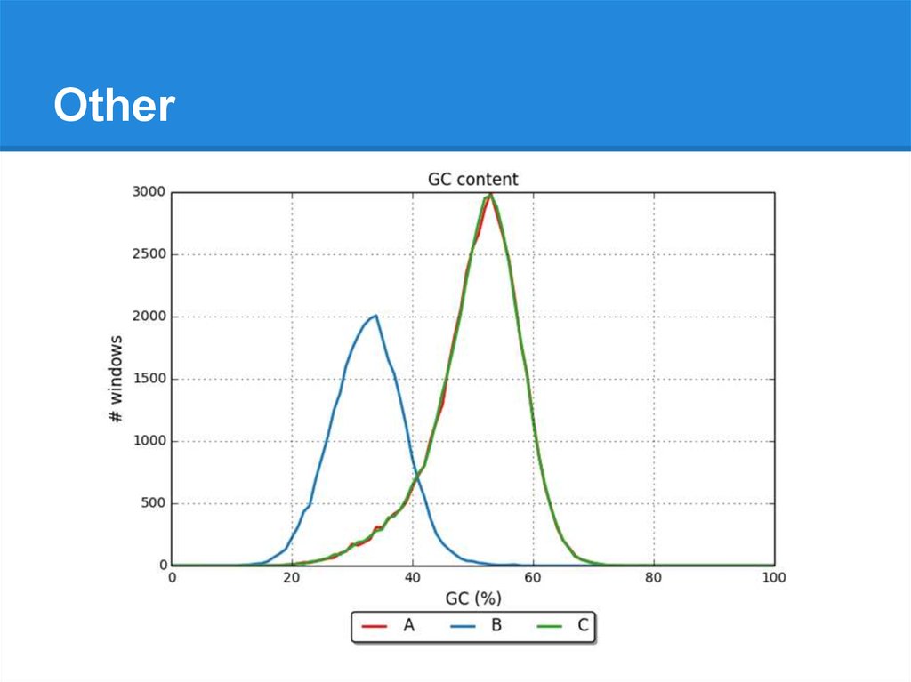
● Distributions of GC % in small windows:
GC=37
GC=44
GC=...
GC=41
60.
Other61.
Reference-based metrics● A lot of metrics
● Accurate assessment
62.
Basic reference statistics● Reference length
● Reference GC %
● Number of chromosomes
63.
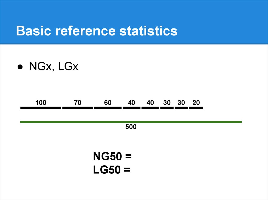
Basic reference statistics● NGx, LGx
100
70
60
40
40
500
NG50 = 40
LG50 = 4
30
30
20
64.
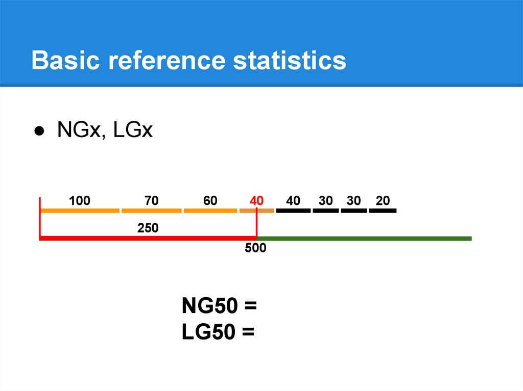
Basic reference statistics● NGx, LGx
100
70
60
40
40
250
500
NG50 = 40
LG50 = 4
30
30
20
65.
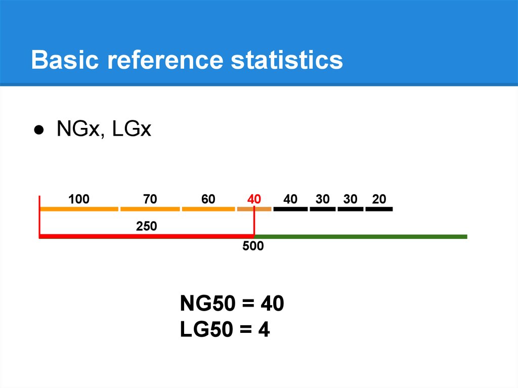
Basic reference statistics● NGx, LGx
100
70
60
40
40
250
500
NG50 = 40 40
LG50 = 4 4
30
30
20
66.
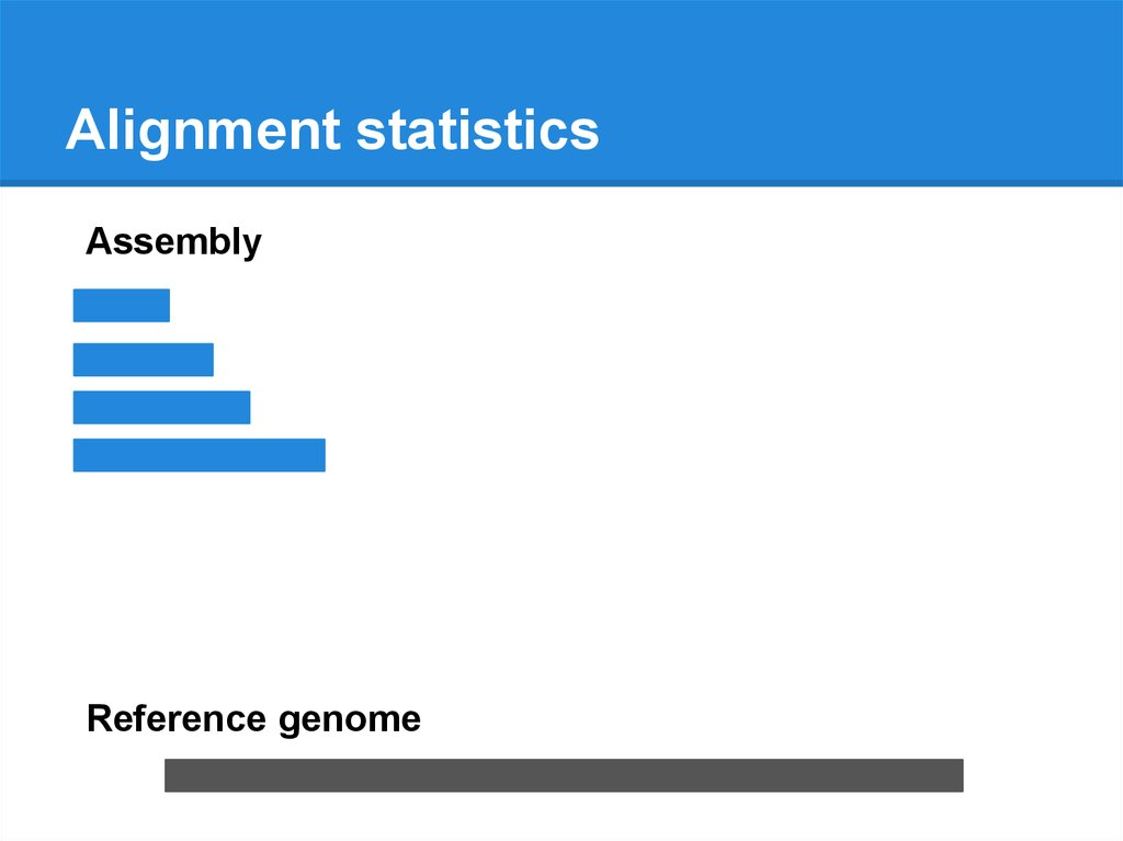
Alignment statisticsAssembly
Reference genome
67.
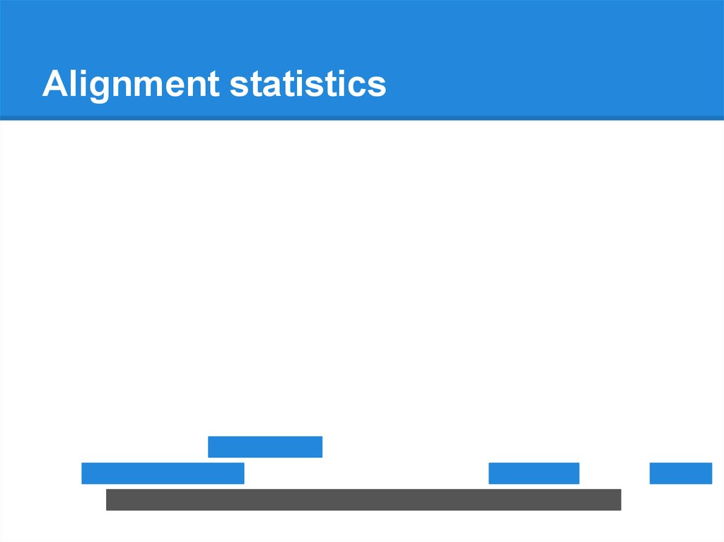
Alignment statistics68.
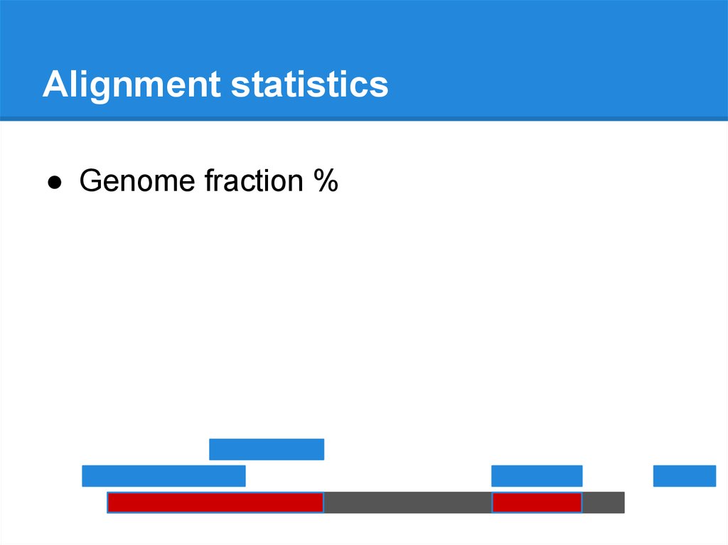
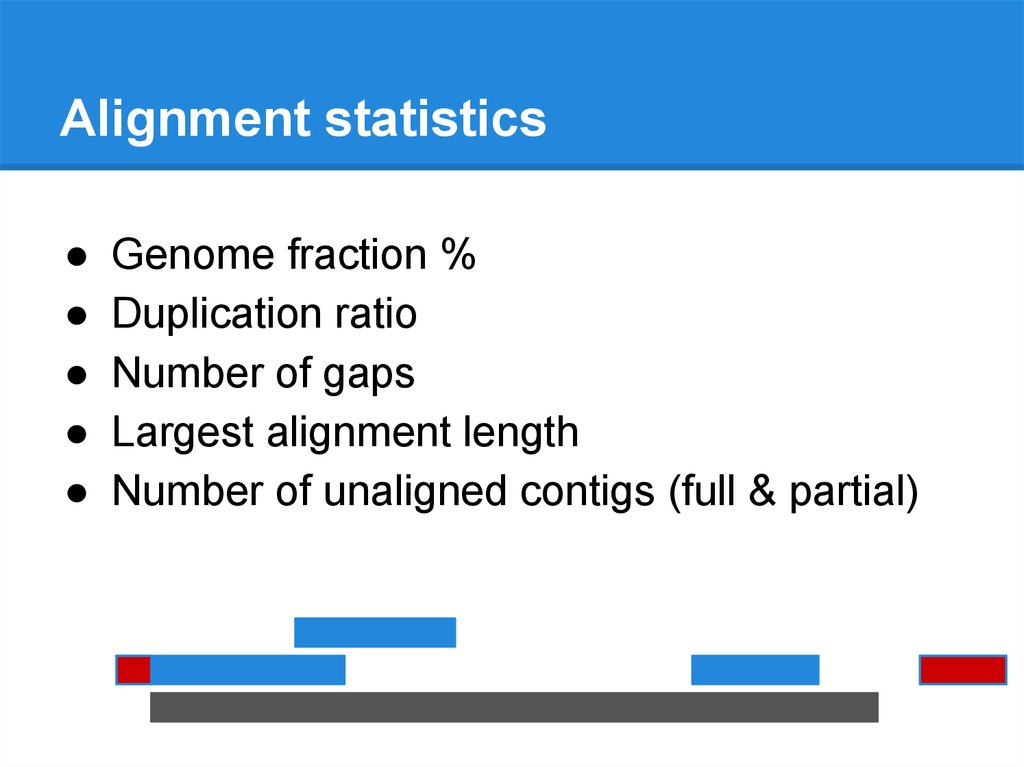
Alignment statistics● Genome fraction %
69.
Alignment statistics● Genome fraction %
● Duplication ratio
70.
Alignment statistics● Genome fraction %
● Duplication ratio
● Number of gaps
71.
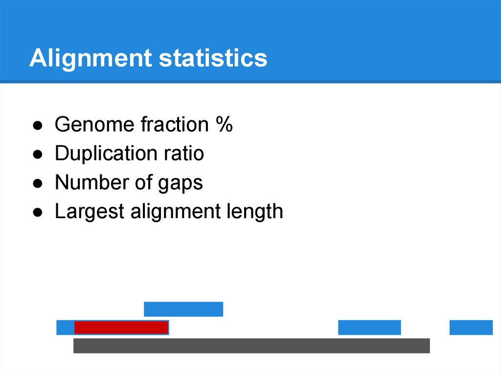
Alignment statisticsGenome fraction %
Duplication ratio
Number of gaps
Largest alignment length
72.
Alignment statisticsGenome fraction %
Duplication ratio
Number of gaps
Largest alignment length
Number of unaligned contigs (full & partial)
73.
Alignment statisticsGenome fraction %
Duplication ratio
Number of gaps
Largest alignment length
Number of unaligned contigs (full & partial)
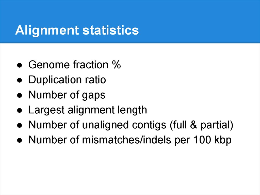
Number of mismatches/indels per 100 kbp
74.
Alignment statisticsGenome fraction %
Duplication ratio
Number of gaps
Largest alignment length
Number of unaligned contigs (full & partial)
Number of mismatches/indels per 100 kbp
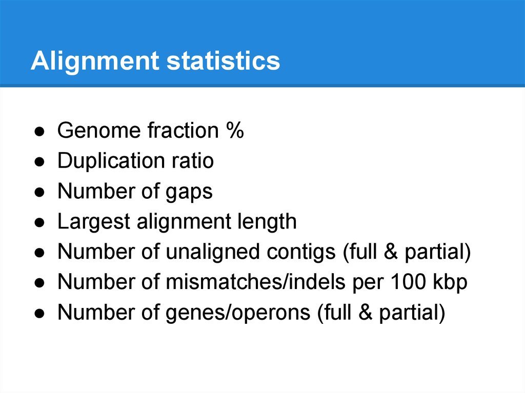
Number of genes/operons (full & partial)
75.
MisassembliesContig
Reference genome
Chromosome 1
Chromosome 2
76.
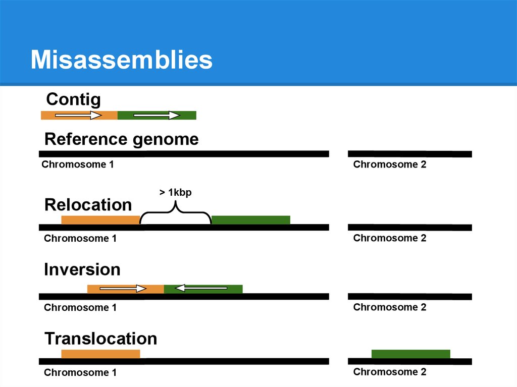
MisassembliesContig
Reference genome
Chromosome 1
Chromosome 2
> 1kbp
Relocation
Chromosome 1
Chromosome 2
Inversion
Chromosome 1
Chromosome 2
Translocation
Chromosome 1
Chromosome 2
77.
NB!There is no best metric
78.
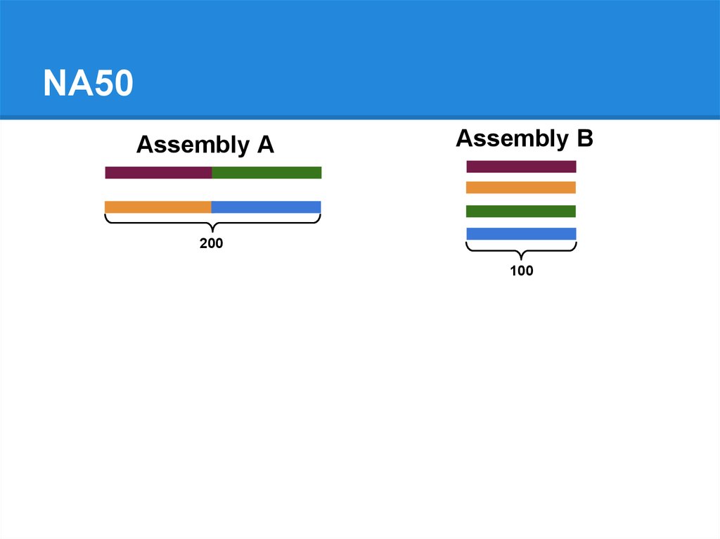
NA50Assembly A
Assembly B
200
100
79.
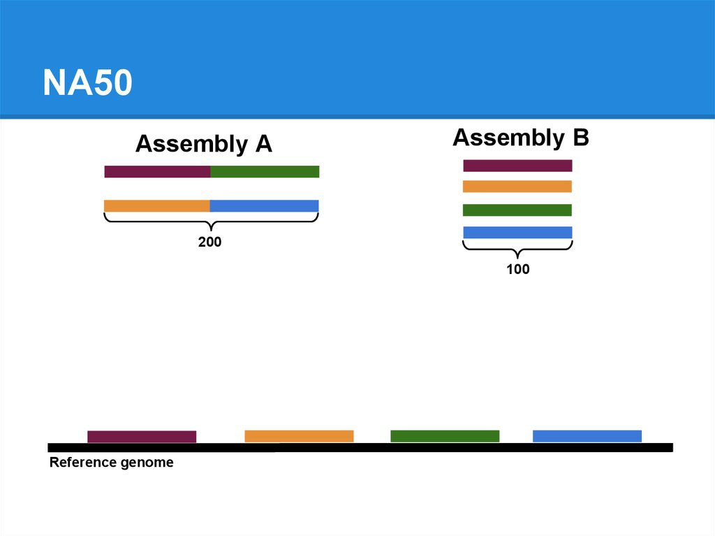
NA50Assembly A
Assembly B
200
100
Reference genome
80.
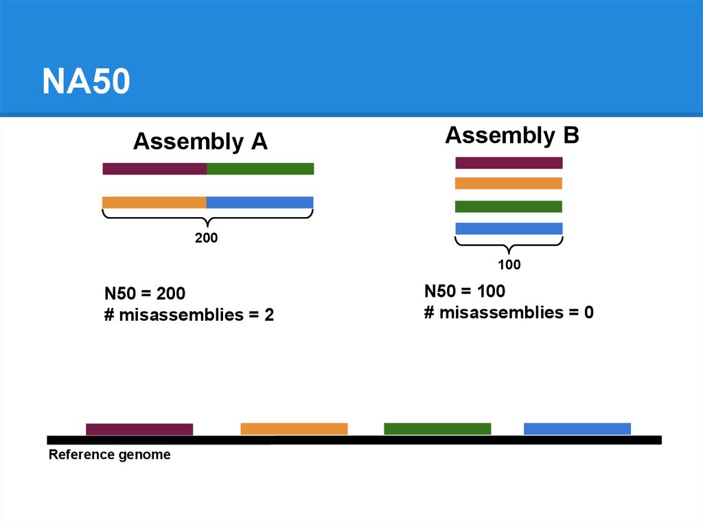
NA50Assembly A
Assembly B
200
100
N50 = 200
# misassemblies = 2
Reference genome
N50 = 100
# misassemblies = 0
81.
NA50Assembly A
Assembly B
200
100
N50 = 200
# misassemblies = 2
NA50 = 100
Reference genome
N50 = 100
# misassemblies = 0
NA50 = 100
82.
QUality ASsesment Toolfor Genome Assemblies
83.
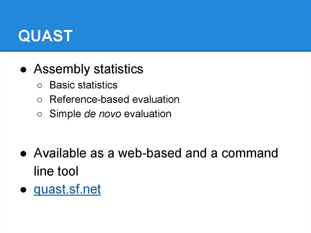
QUAST● Assembly statistics
○ Basic statistics
○ Reference-based evaluation
○ Simple de novo evaluation
● Available as a web-based and a command
line tool
● quast.sf.net
84.
QUAST: console tool● quast.py
● quast.py --help
85.
QUAST basics● quast.py
● quast.py --help
● quast.py contigs.fasta
● quast.py [options] contigs.fasta
● quast.py -o out_dir contigs.fasta
86.
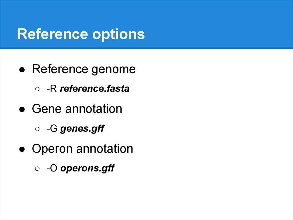
Reference options● Reference genome
○ -R reference.fasta
● Gene annotation
○ -G genes.gff
● Operon annotation
○ -O operons.gff
87.
QUAST output● Reports in different formats
○ Plain text table
○ Tab separated values (Excel, Google Spreadsheets)
○ Interactive HTML
● Plots (PDF/PNG/SVG)
○ Nx, NGx, NAx
○ Genes
○ Cumulative length
● Interactive contig viewers (Icarus)
○ Contig alignment viewer
○ Contig size viewer
88.
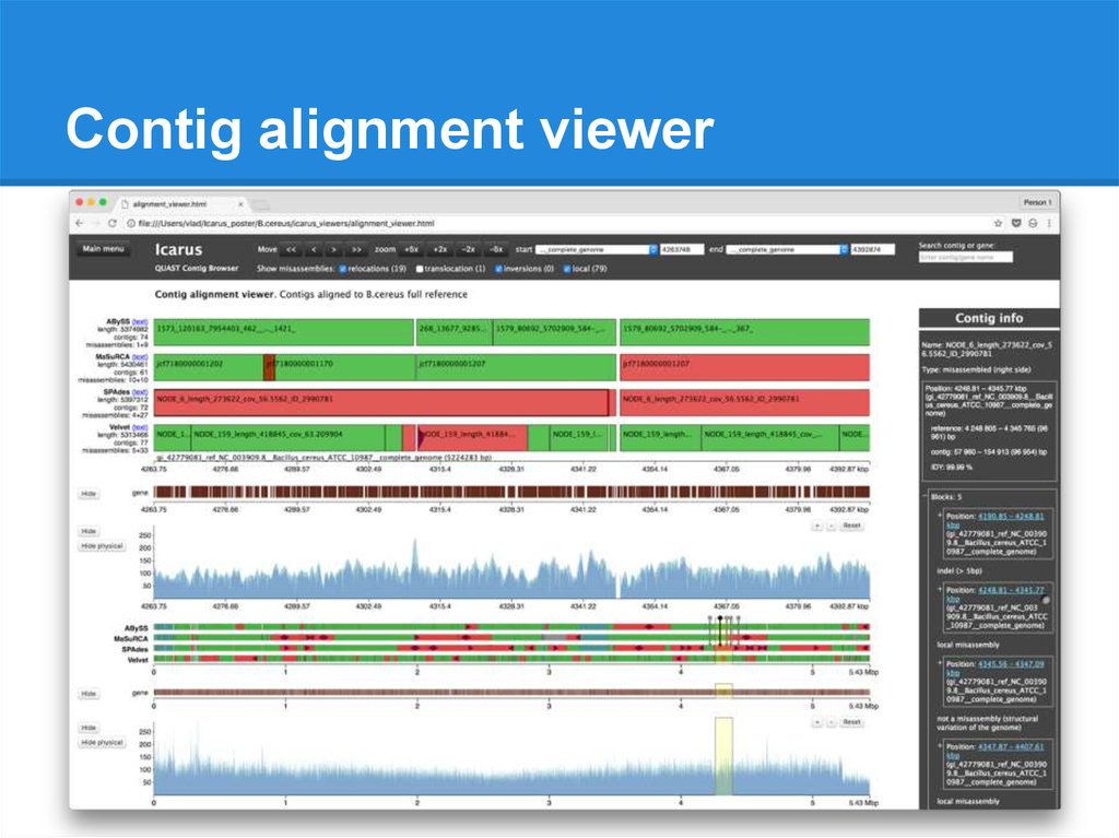
Contig alignment viewer● All alignments for each contig
● Misassembly details
● Contig ordering along the genome
● Overlaps / gaps
89.
Contig alignment viewer90.
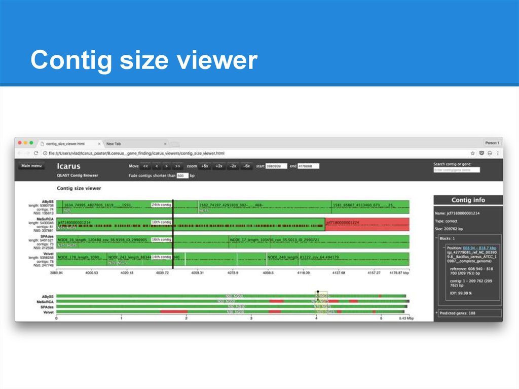
Contig size viewer● Contigs ordered from longest to shortest
● N50, N75 (NG50, NG75)
● Filtration by contig size
● Gene prediction results
● Available without a reference
91.
Contig size viewer92.
De novo evaluation93.
Read-based statistics● Number of aligned/unaligned reads
● % of assembly covered by reads
94.
Read-based statistics● Number of aligned/unaligned reads
● % of assembly covered by reads
● Points with low coverage
● Points with multiple read clipping
● Points with incorrect insert sizes
95.
Annotation-based statistics● Number of ORFs
96.
Annotation-based statistics● Number of ORFs
● Number of gene/operon-like regions
➢ GeneMarkS (Borodovsky et al.)
➢ GlimmerHMM (Majoros et al.)
97.
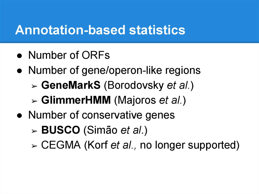
Annotation-based statistics● Number of ORFs
● Number of gene/operon-like regions
➢ GeneMarkS (Borodovsky et al.)
➢ GlimmerHMM (Majoros et al.)
● Number of conservative genes
➢ BUSCO (Simão et al.)
➢ CEGMA (Korf et al., no longer supported)
98.
Thank you!Questions?































 informatics


