Методы исследования взаимодействий с участием белков (Co-IP, equilibrium microdialysis, ITC, MST, SPR, BLI, QСM)

1. Лекция 6 Методы исследования взаимодействий с участием белков (Co-IP, equilibrium microdialysis, ITC, MST, SPR, BLI, QСM).

Примеры.
Случанко Н.Н.

2. Protein-protein interactions (PPIs)

• >80% of proteins function via interaction with other proteins
(PMID: 17640003)
• For each protein ~10 protein partners (interactome)
• Human “interactome” - 300–650 000 PPIs (PMID: 28968506)
• Mechanisms are in the core of the vital processes
• Data are deposited and systematized in databases – MINT, iHOP, InAct
2

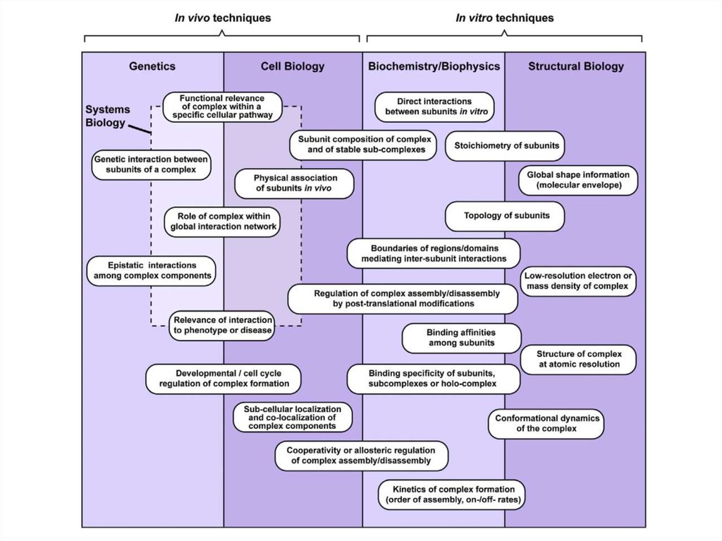
3. Interactions of proteins control the life of the cell

4. Interactions of proteins control the life of the cell

… cell biochemistry would appear to be largely run
by a set of protein complexes, rather than proteins
that act individually and exist in isolated species.
Cell 1992, Bruce Alberts & Miake-Lye

5. Types of PPIs

5

6. Types of PPIs

Homologous interactions:
Heterologous interactions:
• The same proteins
• Different proteins
• Oligomers
• Enzyme – inhibitors
• Coiled-coil
• Antibody – antigen
• Amyloids
• Protein complexes
6

7.

8. Types of PPIs

Qualitative methods:
• Co-immunoprecipitation (Co-IP)
• Pull-down
Quantitative methods:
• Isothermal titration calorimetry (ITC)
https://link.spr
inger.com/boo
k/10.1007%2F
978-1-49392425-7
• Surface plasmon resonanse (SPR)
• Quartz microbalance (QMB)
• Fluorescence polarization (FP)
• others
8

9. Detecting PPI: co-immunoprecipitation (Co-IP)

Protein 1
Protein 2
http://www.piercenet.com
Detect with Ab to 2
(Immunoblot)

10. Reciprocal Co-IP in investigation of 14-3-3 interacting proteins

Reverse
Direct
Immunoprecipitation of 14-3-3 and
detection of bound partner proteins
Immunoprecipitation of partner
proteins and detection of 14-3-3
Ge et al, J.Proteom.Res., 2010: 5848-5858

11. Tandem affinity purification (TAP)

12. M + L <--> ML

M + L <--> ML
M is free macromolecule
L
is free ligand
ML is complex
Case 1 (specific)
Case 2 (general)
Lo >> Mo, Lo=Lfree or you can measure Lfree
hyperbola
Mo * Lfree
ML =
KD + Lfree
parabola
Lo >> Mo, you can’t measure Lfree
KD =
(Mo – ML) * (Lo – ML)
ML
ML = {-(Lo+Mo+KD) +/- √(Lo+Mo+KD)2 - 4MoLo)}/2
https://employees.csbsju.edu/hjakubowski/classes/ch331/bind/olbindderveq.html

13. Simple binding A+B ↔ AB quadratic equation

Online quadratic equation solver:
(just put your numbers for Ao, Bo, KD and choose the right root)
https://www.symbolab.com/solver/equation-calculator/%5Cleft(100x%5Cright)%5Ccdot%5Cleft(10-x%5Cright)-15%5Ccdot%20x%3D0

14. Simple binding A+B ↔ AB quadratic equation

Root 1
Root 2
Online quadratic equation solver:
(just put your numbers for Ao, Bo, KD and choose the right root)
https://www.symbolab.com/solver/equation-calculator/%5Cleft(100x%5Cright)%5Ccdot%5Cleft(10-x%5Cright)-15%5Ccdot%20x%3D0

15. Dimerization process

M + M <==> M2 or D
Kd = [M][M]/[D] = [M]2/[D]
[Mo] = [M] + 2[D]
[M] = [Mo] -2[D]
Kd = (Mo-2D)(Mo-2D)/D
4D2 - (4Mo+Kd)D + (Mo)2 = 0
Y = 2[D]/[Mo]
Lo >> Mo => quadratic equation

16. For a reversible process, one can assess thermodynamics of binding

Kd = 1/Keq
ΔGo = - R T ln Keq = R T ln Kd
@ 20 °C
25 µM = 25*10-6 M
ΔGo = R*T * (-10.6) = – 6.2 kcal/mol
2 cal/mol*K

17. For a reversible process, one can assess thermodynamics of binding

Kd = 1/Keq
ΔGo = - R T ln Keq = R T ln Kd
@ 20 °C
25 nM = 25*10-9 M
ΔGo = R*T * (-17.5) = – 10.3 kcal/mol
2 cal/mol*K

18. ΔGo = R T ln KD

-5.5
@ 20 °C
- 6.2 kcal/mol
-6.0
DGo, kcal/mol
-6.5
-7.0
-7.5
-8.0
-8.5
-9.0
25 mM
-9.5
-10.0
- 10.3 kcal/mol
-10.5
-11.0
0.001
25 nM
0.01
0.1
1
KD, mM
10
100

19. At equilibrium, both forward and reverse reaction rates are equal

kon
Von = Voff
kon [A] [B] = koff [AB]
koff / kon = [A] [B] / [AB] =
koff
Kd = 1/Keq

20. Thermodynamics of interaction

R T ln KD =
Gibbs
free
energy
Enthalpy
Entropy

21. Binding affinity range

http://www.pdbbind-cn.org
1,772,210 binding data :
http://www.bindingdb.org/bind/index.jsp

22. Methods to study PPI (and other interactions!)

Equilibrium microdialysis (EMD)
Fluorescence polarization (FP)
Isothermal titration calorimetry (ITC)
Microscale thermophoresis (MST)
Surface plasmon resonance (SPR)
Biolayer interferometry (BLI)
Quartz crystal microbalance (QCM)

23. Equilibrium microdialysis (EMD)

• Two chambers of equal volume facing each other
• Semipermeable membrane separates the two chambers
• MW cutoff of the membrane allows a ligand to pass through
• Macromolecule with MW higher than cutoff remains in its chamber
• The initial concentrations are known precisely
• The experiment runs till reaching an equilibrium
• At equilibrium, concentrations of L in both chambers are measured
• Parameters of interaction are determined
Chamber 1
M
Chamber 2

24. Equilibrium microdialysis (EMD)

M total is
known
L total is
known
L free is
measured
-> L bound is
calculated

25. Equilibrium microdialysis (EMD)

M + L <--> ML
KD =
[M] * [L]
[ML]
Features
Fast
Easy
Inexpensive
Accurate determination of affinity (KD) and stoichiometry of
interaction
• Membrane type (pore sizes) determines the applicability to
a certain M and L

26. Equilibrium microdialysis (EMD)

Thioflavin T (ThT) binding to acetylcholinesterase (AChE)
AChE
DOI: 10.1021/acschemneuro.8b00111

27. Fluorescence polarization (FP)

The degree of
polarization is associated
with the size of the
particle bearing a
fluorophore

28. Fluorescence polarization (P) or anisotropy (r):

=
2P
3–P
no nominal dependence on dye concentration
P has physically possible values ranging from –0.33 to 0.5 (never achieved)
Typical range 0.01-0.3 or 10-300 mP (P/1000)
Precision is normally 2 mP

29. Fluorescence polarization and molecular size

dyes with various fluorescence lifetimes (τ)
Perrin equation (1926):
Fundamental P (Po) ~0.5 (max)
rotational correlation time of the dye:
Simulation of the relationship between
molecular weight (MW) and fluorescence
polarization (P)
Φ is found to increase by ~1 ns per
2400 Da increase of MW
η = solvent viscosity, T = temperature,
R = gas constant and V = molecular
volume of the fluorescent dye (or its
conjugate)

30. FP features

Great tool to study interactions
Small sample consumption
Low limit of detection
Rapid response
Real-time (not only equilibrium studies)
Kinetic analysis (association/dissociation) is possible
Separation of bound and free species not needed
Good for high-throughput studies

31. FP is very good for high-throughput studies

DOI: 10.1002/1873-3468.13017

32. Isothermal titration calorimetry (ITC)

https://www.youtube.com/watch?v=o_IpWcWKNXI
Sangho Lee (c)

33. Isothermal titration calorimetry (ITC)

Sangho Lee (c)

34. ITC experiment

• Exothermic reaction (common for PPI)
• The sample cell becomes warmer than the reference cell
• Binding causes a downward peak in the signal
• Heat released is calculated by integration under each
peak

35. ITC thermogram

Is calculated
Determined in the experiment
1/KD
stoichiometry
C of
macromolecule in
the cell

36. Small-molecule stabilizer of protein-peptide interaction

Small-molecule stabilizer of proteinpeptide interaction

37. ITC pros and cons

Advantages:
• Ability to determine thermodynamic binding parameters (i.e.
stoichiometry, association constant, and binding enthalpy) in a single
experiment
• Modification of binding partners are not required
Disadvantages:
• Large sample quantity needed
• Kinetics (i.e. association and dissociation rate constants) cannot be
determined
• Limited range for consistently measured binding affinities
• Non-covalent complexes may exhibit rather small binding enthalpies since
signal is proportional to the binding enthalpy
• Slow with a low throughput (0.25 – 2 h/assay), not suitable for HTS

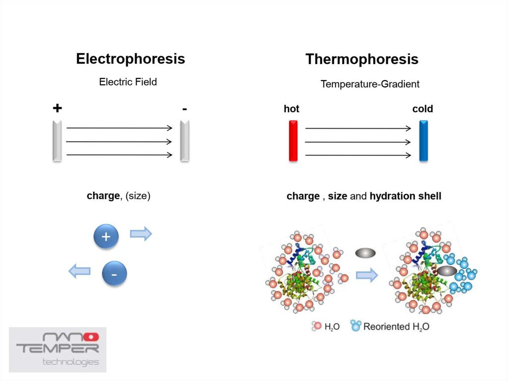
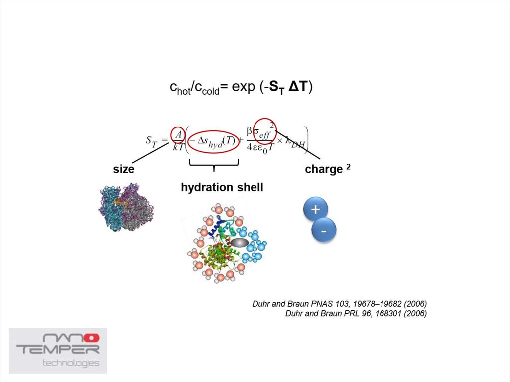
38. Thermophoresis

• The movement of molecules in a temperature gradient

39.

40.

41. Phases of MST experiment

42. Typical MST binding curve

43. Microscale thermophoresis (MST)

https://www.youtube.com/watch?v=rCot5Nfi_Og
https://www.youtube.com/watch?v=4U-0lyHQ0wg

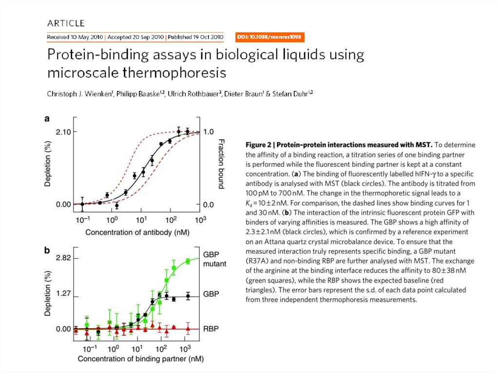
44. MST data examples

45.

46. MST pros and cons

Advantages:
• Small sample size
• Immobilization free
• Minimal contamination of the sample (method is entirely optical and
contact-free)
• Ability to measure complex mixtures (i.e. cell lysates, serum, detergents,
liposomes)
• Wide size range for interactants (ions to MDa complexes)
Disadvantages:
• Hydrophobic fluorescent labelling required, may cause non-specific
binding
• No kinetic information (i.e. association and dissociation rates)
• Highly sensitive to any change in molecular properties

47. Surface plasmon resonance (SPR)

48. Reflection and refraction at different angles

49. Surface plasmon resonance (SPR)

https://www.youtube.com/watch?v=sM-VI3alvAI
https://www.youtube.com/watch?v=oUwuCymvyKc
https://youtu.be/o8d46ueAwXI
Patching, Biochim. Biophys. Acta (2014)

50. SPR sensorgram

51. Chips

Biacore

52. Why is kinetic analysis important?

53. Practical considerations

• Use several concentrations (ideally, 10 times below till 10
times above KD)
• Accurate protein concentration must be determined
• Zero concentration should also be included
https://www.youtube.com/watch?v=e_tNkxbE2kY

54. Data analysis by simultaneous fitting of all curves using a binding model

Biacore

55. Steady-state and kinetic ways to determine affinity (KD)

Biacore

56. Steady-state and kinetic ways to determine affinity (KD)

Biacore

57. SPR pros and cons

Advantages:
• Label-free detection
• Real-time data (i.e. quantitative binding affinities, kinetics and
thermodynamics)
• Medium throughput
• Sensitivity and accuracy
• Measures over a very wide range of on rates, off rates and affinities
• Small sample quantity
Disadvantages:
• Expensive instrument and sensors
• Expensive maintenance
• Steep learning curve
• Specialized technician or senior researcher required to run experiments
• Immobilization of one of the binding partners required

58. Biolayer interferometry (BLI)

https://www.moleculardevices.com/applications/biologics/b
li-technology#gref
ForteBio; Citartan et al. Analyst (2013)

59. Instruments

8 channels
1 channel

60. Instruments

4ul
8 channels
1 channel

61. BLI sensorgrams

Key Benefits of BLI
• Label-free detection
• Real-time results
• Simple and fast
• Improves efficiency
• Crude sample
compatibility
Exemplary studies:
https://journals.plos.org/plosone/article?id=10.1371/journal.pone.0106882
https://www.ncbi.nlm.nih.gov/pmc/articles/PMC4089413/

62. BLI pros and cons

Advantages:
• Label-free detection
• Real-time data
• No reference channel required
• Crude sample compatibility
• Fluidic-free system so less maintenance needed
Disadvantages:
• Immobilization of ligand to surface of tip required
• No temperature control
• Low sensitivity (100-fold lower sensitivity of detection compared to SPR)

63. ITC vs SPR and BLI comparison

64. Quartz crystal microbalance (QCM)

High frequent oscillations of the quartz crystal (5-10 MHz) with the Au chip
Mass detection with super accuracy – quartz crystal resonator senses ~1 Hz
Upon mass deposition on the QCM sensor, the frequency decreases
Sensitivity can be ~ 20 ng/cm2 per Hz
Low throughtput, rather rare method
Sample volume 50-200 ul
Label-free
Xdelic
Sauerbrey equation:
freq change
mass change
sensitivity
https://www.youtube.com/watch?v=xDKOUpSR3EQ
https://openqcm.com/openqcm

65. Microfluidics delivers the sample and the deposited mass fraction is measured

https://www.youtube.com/watch?v=xDKOUpSR3EQ

66. Overview of the course

Proteins: size and hydrodynamic parameters
Identification of proteins by their sequence
Spectroscopy methods
Stability of proteins
Protein structure – high resolution methods
Protein structure – low resolution methods
Interactions involving proteins