


 mathematics
 finance
Similar presentations:
")
")
")
")
")
")


Simultaneous games. Oligopoly. (Lecture 2)
1. Lecture 2 Simultaneous games: Oligopoly
2. Oligopoly
2Extreme forms of market structure are uncomplicated:
Monopoly: one producer, no strategic interaction
Perfect competition: many producers, price is given, no
strategic interaction
Oligopoly: the industry is dominated by a small number of
large firms. Intermediate case, between perfect competition
and monopoly.
Smartphones industry
Oil producers
Accounting Big 4
Boeing and Airbus
3. Strategic interactions and oligopoly
3Strategic interactions and
oligopoly
When making strategic decisions (on prices, quantity,
advertising, innovation etc.) the oligopolist must consider
the actions/reactions of its competitors.
Payoff interdependency: A producer’s payoff depends
on what the other producers do.
Use of game theory.
Application of NE to oligopoly theory. Analysis of the
decision of how much to produce (quantity).
4. Demand and costs
4Demand: The market price is a function of the total
quantity produced in the industry, e.g:
P (Q) 1 0.001Q
Q 400 P 0.6
e.g:
Costs: Suppose that the marginal cost is 0.28
5. Monopoly
5The monopolist chooses Q to maximize profit:
M Q(1 0.001Q) 0.28Q 0.72Q 0.001Q 2
M
0 0.72 0.002Q 0 Q 360
Q
Outcome: Q 360
P 0.64
M 129.6
Low output to keep prices high and maximize profit.
6. Perfect competition
6Many producers, the price is given.
In equilibrium, Q is such that P=MC, i.e. P=0.28.
Producers make zero profit.
P = 1 − 0.001Q = 0.28, hence Q = 720,
Quantity is higher under perfect competition than
under monopoly.
7. The Cournot model
7What is the Cournot model?
Two producers, Firm 1 and Firm 2 (oligopoly).
Model of industry structure where producers’ strategic
decision is about how much to produce.
Produce the same good
Sell on the same market
One market price, which depends on the total output
No entry
Simultaneous game
Example: oil producing countries
8. Demand
The more producers jointly produce, the lower the marketprice
Q q1 q2
P (q1 q2 ) 1 0.001(q1 q2 )
Example: q1 q2 200 Q 400 P 0.6
9. Costs and profit
9Suppose that the marginal cost is 0.28:
C1 (q1 ) 0.28 q1
C (q ) 0.28 q2
Profit of Firms 1 and 2:
2
2
1 q1 P(q1 q2 ) C1 (q1 )
2 q2 P(q1 q2 ) C2 (q2 )
10. Discrete choices
Suppose there are just three possible quantities that eachfirm i=1,2 can choose qi = 180, 240 or 360.
There are 3x3=9 possible outcomes. For example, if firm 1
chooses q1=180, and firm 2 chooses q2=240, then:
P(180 240) 1 0.001 420 0.58
1 180 0.58 0.28 180 54
2 240 0.58 0.28 240 72
11. Discrete choices
Nash Equilibriumq1=18
0
Firm 1 q1=24
0
q1=36
0
Firm 2
q2=18 q2=24 q2=36
0
0
0
64.8 , 64.8
54, 72
32.4, 64.8
72, 54
57.6, 57.6
28.8, 43.2
64.8, 32.4
43.2, 28.8
0, 0
12. Continuous choices
12Discrete games are not suitable to analyze the
decision of how much to produce
Producers are not limited to just 3 levels of production.
Quantity is a continuous variable, not a discrete one.
We now assume that producers can produce any
quantity.
How much to produce?
More units sold means more volume, but lower price.
Essential to take into account the other producer’s behavior.
13. Continuous choices
13Simplifying the profit function:
1 q1 P(q1 q2 ) C1 (q1 )
1 q1 (1 0.001 (q1 q2 )) 0.28q1
2
1 0.72q1 0.001q1 0.001q1q2
2
2 0.72q2 0.001q2 0.001q1q2
14. Best responses
14We find the Nash equilibrium by deriving the best
response functions.
To maximize profit, differentiate and set equal to
zero:
1
0.72 0.002q1 0.001q2 0
q1
q1 360 0.5q2
Firm 1’s best response
Do the same for Firm 2:
q2 360 0.5q1
Firm 2’s best response
15. Best responses
15Firm 1 believes Firm 2
will sell q2:
Firm 1’s profitmaximizing q1 is:
0
360
100
310
200
260
240
240
300
210
360
180
400
160
720
0
16. Best responses
16q2
720
q1 360 0.5q2
The more Firm 2 produces, the lower the market
price, and the less Firm 1 chooses to produce.
0
q1
360
17. Best responses
17q2
The more Firm 1 produces, the lower the market
price, and the less Firm 2 chooses to produce.
360
q2 360 0.5q1
Firm 2’s best response
720
q1
18. Nash equilibrium
18Nash Equilibrium is where best responses meet.
Firm 1’s equilibrium strategy is his best response to
Firm 2’s equilibrium strategy which is also his best
response to Firm 1’s equilibrium strategy.
Joint best response, and no incentive for producers to
choose a different action.
q1 360 0.5q2 360 0.5(360 0.5q1 ) 180 0.25q1
q1 240
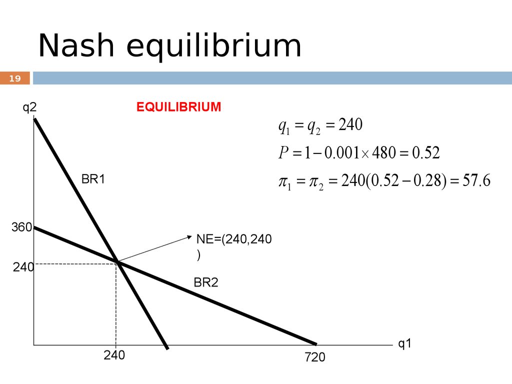
19.
Nash equilibrium19
q2
EQUILIBRIUM
q1 q2 240
P 1 0.001 480 0.52
1 2 240(0.52 0.28) 57.6
BR1
360
NE=(240,240
)
240
BR2
240
720
q1
20. Nash equilibrium
20q2
• Convergence towards Nash equilibrium:
• Why are other production levels not equilibrium?
• Start from (0,360)
BR1
360
BR2
0
720
q1
21. Effect of market structure
21Monopoly
Cournot
Perfect
competiti
on
Industry
Output
360
480
720
Price
Industry
Profit
0.64
129.6
0.52
115.2
0.28
0
Oligopoly delivers an intermediary outcome between two
extreme forms of market structure.
22. Effect of market structure
22Cournot with more than 2 producers:
Produce
rs
Price
q per
firm
Profit
per
firm
Industr Industr
yQ
y profit
2
0.52
240
57.6
480
115.2
3
0.46
180
32.4
540
97.2
10
0.34
65.5
4.3
654
42.8
100
0.28
7.1
0.05
712
5.1
23. Effect of market structure
23Having fewer producers is associated with:
Lower total output
Higher prices
Higher profitability
Empirical evidence shows that profitability is on
average higher in highly concentrated industries.
24. Cartel
24Wouldn’t the two producers be better off cooperating rather
than competing? YES
Both producers could maximize joint profit by jointly
producing the monopolist output level: Q=360, i.e. 180 for
each producer.
The monopolist profit (129.6) is then shared between the two
producers (i.e. 64.8 for each, instead of 57.6 if they play the
NE).
25. Cartel
25“The OPEC cartel agreed on Wednesday to reduce production by
2.2 million barrels a day, the group’s largest cut ever, in an effort
to put a floor on falling oil prices.
…Mr. Khelil (OPEC’s president) said the group wanted to
“eliminate” an overhang of oil inventories …and aimed to push
prices up to $70 to $80 a barrel.
“We have…excessive stocks that could really lead to a collapse
in prices,” Mr. Khelil said during a chaotic and confused news
conference after the meeting.
(NY Times, December 17, 2008)
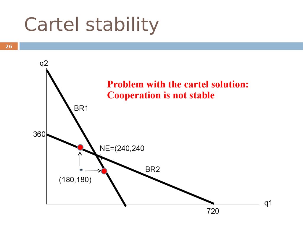
26.
Cartel stability26
q2
Problem with the cartel solution:
Cooperation is not stable
BR1
360
NE=(240,240
)
BR2
(180,180)
720
q1
27. Cartel stability
27Each producer makes more profit by deviating from the
cartel quantity. For instance, if Firm 1 sticks to the cartel
quantity of 180, Firm 2’s best response is:
q2 360 0.5 x180 270
2 72.9
The cartel problem is a Prisoner’s dilemma situation: it is
collectively rational to cooperate (“optimal” outcome), but
it is individually rational to defect (NE).
28. Cartel stability
28“The coffee bean cartel, the Association of Coffee
Producing Countries, whose members produce 70% of
the global supply, will shut down in January after
failing to control international prices. [...] Mr Silva also
said the failure of member countries to comply with the
cartel’s production levels was a reason for the closure.”
(BBC News, October 19, 2001)
29. Cartel stability
29To summarize…
Producers have incentive to form cartels, but cartels are
unstable.
Q: How to explain the fact that some cartels are quite
stable, unlike what is predicted in the Cournot model?
List of cartel violations in the European Union
http://ec.europa.eu/competition/cartels/cases/cases.html
30. Comparative statics
30If Firm 1’s marginal cost is 0.25 rather than 0.28, how does
it affect the outcome?
C1 (q1 ) 0.25 q1
Equilibrium:
q1 260
q2 230
P 0.51
1 67.6
2 52.9
Increase of 17%
31. Summary
31Nash equilibrium and continuous choices.
Oligopoly and quantity competition: Cournot model.
Trade-off between high output and low price, or low
output and high price.
Strategic interactions yield a unique NE, with
intermediate output level.
The cartel solution is more profitable but not stable.