


 mathematics
Similar presentations:


")


Survey. Factors that affecton shopping centers selection
1. Survey
SURVEYFA C TO R S T H AT A F F E C T O N
SHOPPING CENTERS SELECTION
2. Y=ß0+ ß1X1+ ß2X2+ ß3x3+ ß4x4+ ß5x5+ ß6x6+ ß7x7+ ß8x8+ ß9x9 There are:
Y=ß0+ ß1X1+ ß2X2+ ß3X3+ ß4X4+ ß5X5+ ß6X6+ß7X7+ ß8X8+ ß9X9
THERE ARE:
• Y-your favorite shopping center
X7-game library
• X1-age
• X2-location
X8-area
• X3-raiting
X9-price
• X4-number of boutiques
• X5-advice from friends
• X6-design
3. Regression
REGRESSIONSource |
SS
df
MS
• -------------+------------------------------
Number of obs =
F( 3, 47) =
1.23
Model | 7.26303807
3 2.42101269
Prob > F
Residual | 92.4232364
47 1.96645184
R-squared
• -------------+-----------------------------
Total | 99.6862745
50 1.99372549
51
= 0.3089
= 0.0729
Adj R-squared = 0.0137
Root MSE
= 1.4023
-----------------------------------------------------------------------------Y|
Coef.
Std. Err.
t P>|t| [95% Conf. Interval]
-------------+---------------------------------------------------------------X2 | 0.2046206 0.2961503 -0.69 0.493 -.8003982 .391157
X5 | 0.1337833 0.1293437 -1.03 0.306 -.3939893 .1264227
X8 | 0.2717567 0.1853627 -1.47 0.149 -.6446583 .1011449
_cons | 4.694907 1.465329 3.20 0.002 1.747045 7.642769
4. Y= 4.694907 +0.204*X2+0,133*X5+0,271*X8
When all the independent variables are equal to zero, the intercept of the model is 4.694907When 1 increase in X2 and hold second independent constant, satisfaction rate will increase by
0.2046206
When 1 increase in X5 and hold another independent constant, dependent variable will increase
by 0,1337833
When 1 increase in X6 and hold second independent constant,satisfaction rate will increase by
0,2717567.
5. T-test
T-TESTa)H0: β2=0 no linear relationship
H1: β2≠0 linear relationship does exist between x and y
t= (β2-0)/se(β2)= 0.2046206/0.2961503= 0.69
T=(0,025,3)=3,182
t<T, therefore we fail reject at 5% significance level and conclude that β2 is statistically
insignificance at 10% level
6. T-test
T-TESTb) H0: β5=0 no linear relationship
H1: β3≠0 linear relationship does exist between xj and y
t= | 0.1337833/0.1293437= 1,0343
T(0,025,2)=3,182
t<T, therefore we fail reject at 5% significance level and conclude that β3 is statistically
insignificance at 10% level
7. T-test
T-TESTc) H0: β8=0 no linear relationship
H1: β6≠0 linear relationship does exist between x and y
t= 0.2717567/0.1853627= 1,466088082424
t<T, therefore we fail reject at 5% significance level and conclude that β4 is statistically
insignificance at 10% level
8. F-test
F-TESTH0: β2=β5=β8=0
H1: at least one of the βi is not equal to zero
f-statistics=1.23
F( 3, 47) =2.201
9. R-Square, R2.
R-SQUARE, R2.The value of R2 is 0,01 means that 1% of the variation in satisfaction rate can be
explained by the variation of reputation, social life rate, building, feedback,
accreditation.
10. Auto Correlation
• Breusch-Godfrey LM test for autocorrelation• --------------------------------------------------------------------------
lags(p) |
chi2
df
Prob > chi2
• -------------+------------------------------------------------------------
1
|
0.142
1
0.7067
• ---------------------------------------------------------------------------
H0: no serial correlation
11. Hetrocodeceticity test
HETROCODECETICITY TEST• Breusch-Pagan / Cook-Weisberg test for heteroskedasticity
Ho: Constant variance
Variables: fitted values of Y
chi2(1)
Prob > chi2 = 0.8364
=
0.04
12. Durbin-Watson test
DURBIN-WATSON TEST• Durbin-Watson d-statistic( 4, 51) = 1.857508
• 0-----------------dl(1.206)---------------------du(1.537)------------4-du(2.463)--------------4-dl(2.79)--------------4
• P
• No autocorrelation
?
Nope
?
Negative
13. Normality test
0.1
Density
.2
.3
• Jarque-Bera normality test: 3.129 Chi(2) 0.2092
-2
-1
0
Residuals
1
2
3
14. Multicolenarity test
MULTICOLENARITY TEST• Variable |
VIF
1/VIF
• -------------+---------------------
X5 |
1.07
0.937834
X2 |
1.04
0.957690
X8 |
1.02
0.978161
• -------------+---------------------
Mean VIF |
1.04
15. Ramsey test
RAMSEY TEST• Ramsey RESET test using powers of the fitted values of Y
Ho: model has no omitted variables
F(3, 44) =
Prob > F =
0.01
0.9980
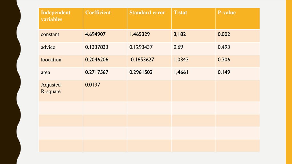
16.
Independentvariables
Coefficient
Standard error
T-stat
P-value
constant
4.694907
1.465329
3,182
0.002
advice
0.1337833
0.1293437
0.69
0.493
loocation
0.2046206
0.1853627
1,0343
0.306
area
0.2717567
0.2961503
1,4661
0.149
Adjusted
R-square
0.0137
17. Histogram
00
.1
.5
.2
1
2
X2
3
4
5
.3
Density
1
.4
1.5
.5
HISTOGRAM
1
2
Y
3
4
5
18. Histogram
00
.2
.2
.4
1
2
X8
3
4
5
.4
Density
.6
.6
.8
.8
1
HISTOGRAM
1
2
X5
3
4
5