


 informatics
Similar presentations:


")
")


Modeling of nonstationary time series using nonparametric methods
1.
Modeling of nonstationary time seriesusing nonparametric methods
Fedorov Sergei Leonidovich
2.
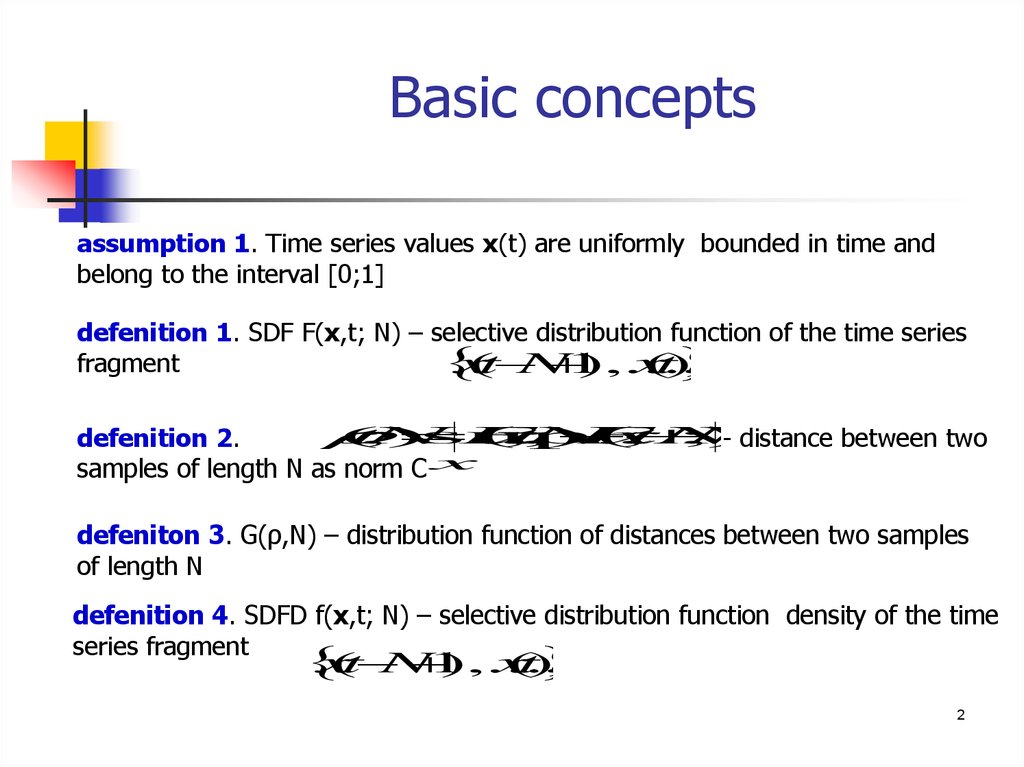
Basic conceptsassumption 1. Time series values x(t) are uniformly bounded in time and
belong to the interval [0;1]
defenition 1. SDF F(x,t; N) – selective distribution function of the time series
fragment
x
(
t
N
1
),...,
x
(
t)
(
t
;
N
)
sup
F
(
x
,
t
;
N
)
F
(
x
,
t
N
;
N
)
defenition 2.
- distance between two
samples of length N as norm C x
defeniton 3. G(ρ,N) – distribution function of distances between two samples
of length N
defenition
4. of
SDFD
f(x,t;
N) – selective
distribution
function
the time
The SS
in the norm
C for
stationary
VDFs does
not depend
on thedensity
type ofofdistribution
fragment
and isseries
calculated
from the Kolmogorov function
x
(
t
N
1
),...,
x
(
t)
2
3.
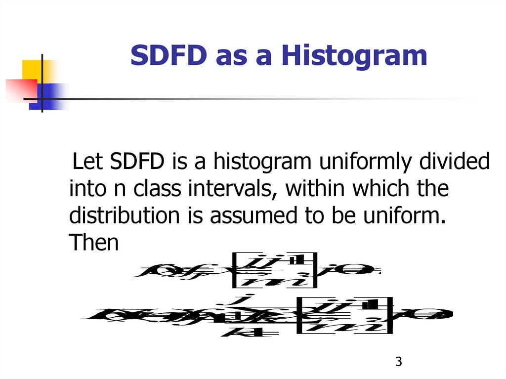
SDFD as a HistogramLet SDFD is a histogram uniformly divided
into n class intervals, within which the
distribution is assumed to be uniform.
Then
jj
1
f
(
x
)
f
,
x
;
,j
0
n
1
j
n
n
j
j
j
1
F
(
x
)
(
nx
j
)
f
f
,
x
;
,j
0
n
1
j
1
k
n
n
k
1
3
4.
Solved problemsDeveloping of a nonparametric indicator of a
breakdown for a selective distribution function
in a sliding window;
Creating of a model of distribution function
evolution using the empirical kinetic equation;
Developing of the method of stochastic process
trajectories set generation.
4
5.
Practical use• Earthquake research
• Medicine
• Text analysis
• Telecommunications
• Stocks market
5
6.
Why is it important to take in accountthe non stationary nature of the
series
All theorems for estimating the confidence interval are
proved only for the stationary case
6
7.
The classical theorems onconvergence
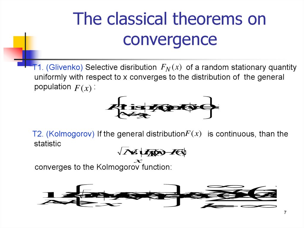
Т1. (Glivenko) Selective disribution FN (x) of a random stationary quantity
uniformly with respect to x converges to the distribution of the general
population F (x) :
P
lim
sup
F
(
x
)
F
(
x
)
0
1
N
N
x
Т2. (Kolmogorov) If the general distributionF (x) is continuous, than the
statistic
N
sup
F
(
x
)
F
(
x
)
N
x
converges to the Kolmogorov function:
k 2
2
lim
P
0
N
sup
F
(
x
)
F
(
x
)
z
K
(
z
)
(
1
)
exp
2
k
z
N
N
x
k
7
8.
Methods of the nonstationary time series analysis1.
Ordinary least squares.
2.
Time series cointegriation, i. e. the linear combination of these series
becomes stationary. (Boks-Dzhenkins, 1972).
3.
Autoregressive models (Dickey-Fuller, 1979).
4.
Adaptive models of time series: multiparameter models of short-term
forecasting(Holt,Winters, 1990-2000).
All these models operate directly with the elements of the series
and predict its values. The distribution function of the series
is not studied. The results depend on the length of the
sample and the current time.
8
9.
Nonparametric comparison ofsamples
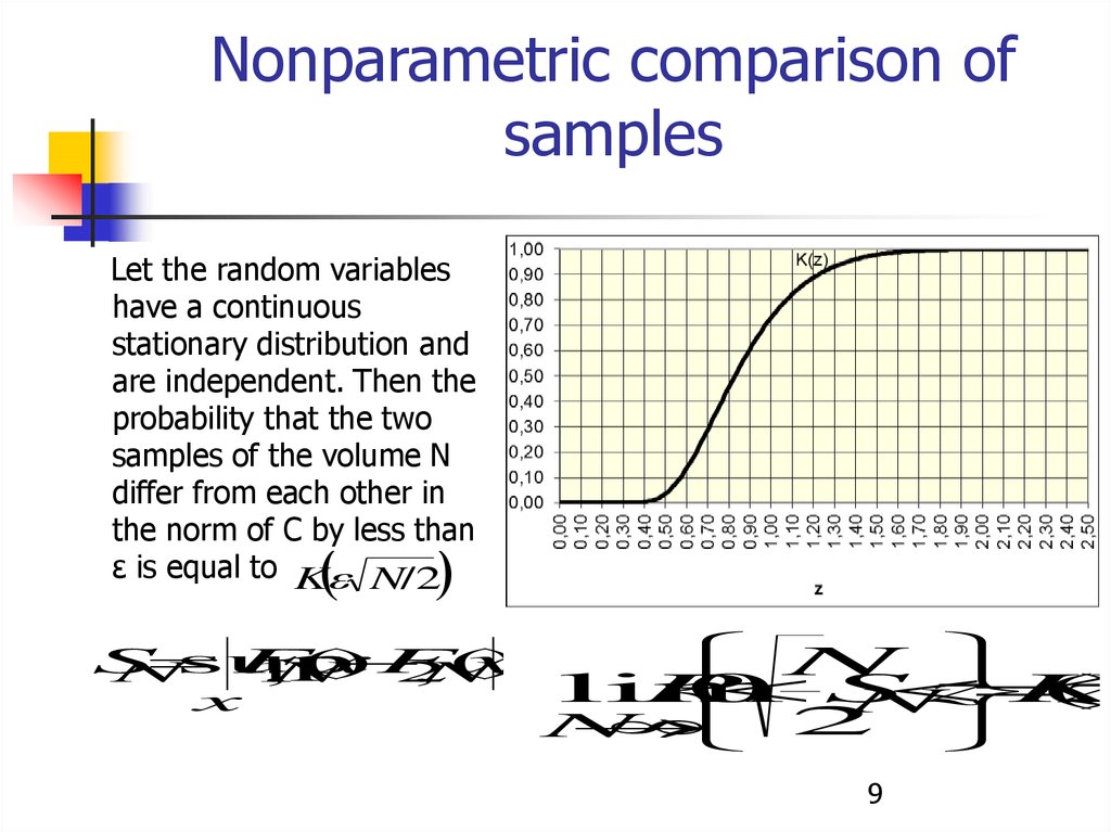
Let the random variables
have a continuous
stationary distribution and
are independent. Then the
probability that the two
samples of the volume N
differ from each other in
the norm of C by less than
ε is equal to K N/2
S
sup
F
(
x
)
F
(
x
)
N
1
,
N
2
,
N
x
N
lim
P
0
S
z
K
(
z
)
N
N
2
9
10.
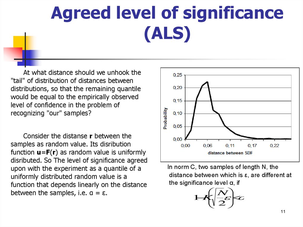
Agreed level of significance(ALS)
At what distance should we unhook the
"tail" of distribution of distances between
distributions, so that the remaining quantile
would be equal to the empirically observed
level of confidence in the problem of
recognizing "our" samples?
Consider the distanse r between the
samples as random value. Its disribution
function u=F(r) as random value is uniformly
disributed. So The level of significance agreed
upon with the experiment as a quantile of a
uniformly distributed random value is a
function that depends linearly on the distance
between the samples, i.e. α = ε.
In norm C, two samples of length N, the
distance between which is ε, are different at
the significance level α, if
N
1 K
2
11
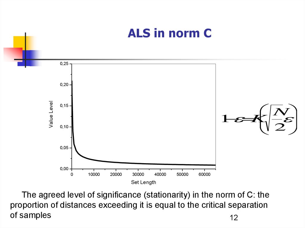
11.
ALS in norm C0,25
Value Level
0,20
N
1
K
2
0,15
0,10
0,05
0,00
0
10000
20000
30000
40000
50000
60000
Set Length
The agreed level of significance (stationarity) in the norm of C: the
proportion of distances exceeding it is equal to the critical separation
of samples
12
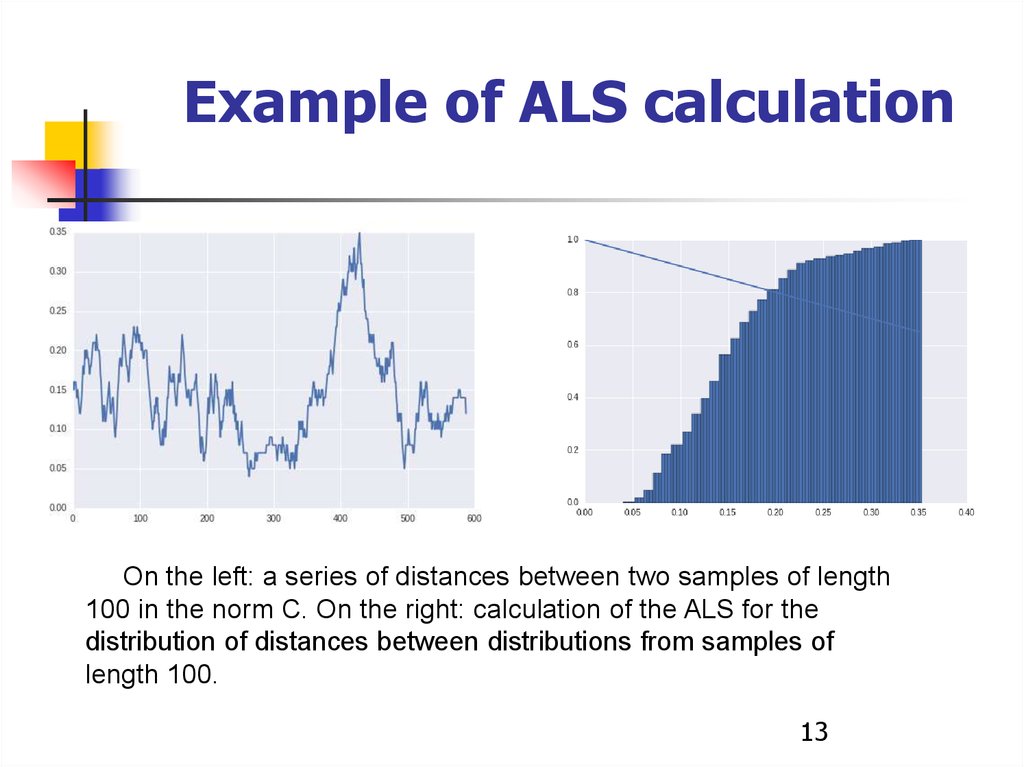
12.
Example of ALS calculationOn the left: a series of distances between two samples of length
100 in the norm C. On the right: calculation of the ALS for the
distribution of distances between distributions from samples of
length 100.
13
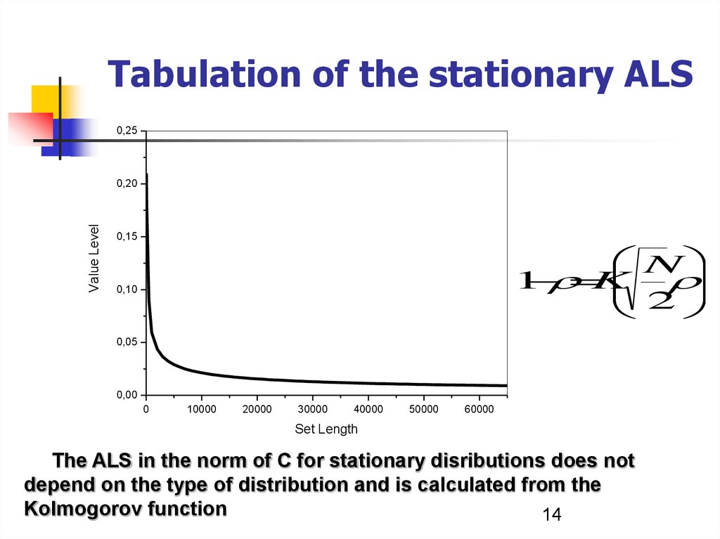
13.
Tabulation of the stationary ALS0,25
Value Level
0,20
0,15
N
1
K
2
0,10
0,05
0,00
0
10000
20000
30000
40000
50000
60000
Set Length
The ALS in the norm of C for stationary disributions does not
depend on the type of distribution and is calculated from the
Kolmogorov function
14
14.
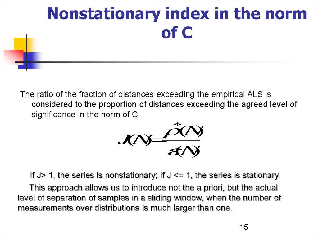
Nonstationary index in the normof C
The ratio of the fraction of distances exceeding the empirical ALS is
considered to the proportion of distances exceeding the agreed level of
significance in the norm of C:
(N
)
J(N
)
(N
)
*
If J> 1, the series is nonstationary; if J <= 1, the series is stationary.
This approach allows us to introduce not the a priori, but the actual
level of separation of samples in a sliding window, when the number of
measurements over distributions is much larger than one.
15
15.
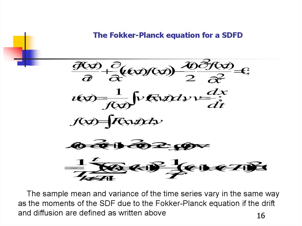
The Fokker-Planck equation for a SDFD2
f(x
,t)
(t)
f(x
,t)
u
(x
,t)f(x
,t)
0
;
2
t
x
2
x
1
dx
u
(x
,t)
vF
(x
,v
,t)dv
, v ;
f(x
,t)
dt
f(x
,t)
(x
,v
,t)dv
;
F
2
2
(
t
)
(
t
1
)
(
t
)
2
cov
(
t
)
x
,
u
1t
21
2
x
(
k
)
x
(
k
1
)
x
(
t
1
)
x
(
t
T
1
)
0
2
T
T
k
t
T
1
The sample mean and variance of the time series vary in the same way
as the moments of the SDF due to the Fokker-Planck equation if the drift
and diffusion are defined as written above
16
16.
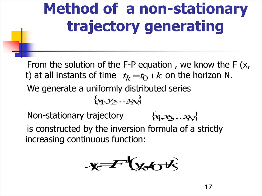
Method of a non-stationarytrajectory generating
From the solution of the F-P equation , we know the F (x,
t) at all instants of time tk t0 k on the horizon N.
We generate a uniformly distributed series
y1,y2,...,
yN
Non-stationary trajectory
x1,x2,...,
xN
is constructed by the inversion formula of a strictly
increasing continuous function:
x
F y
,t0
k
k
k
1
17
17.
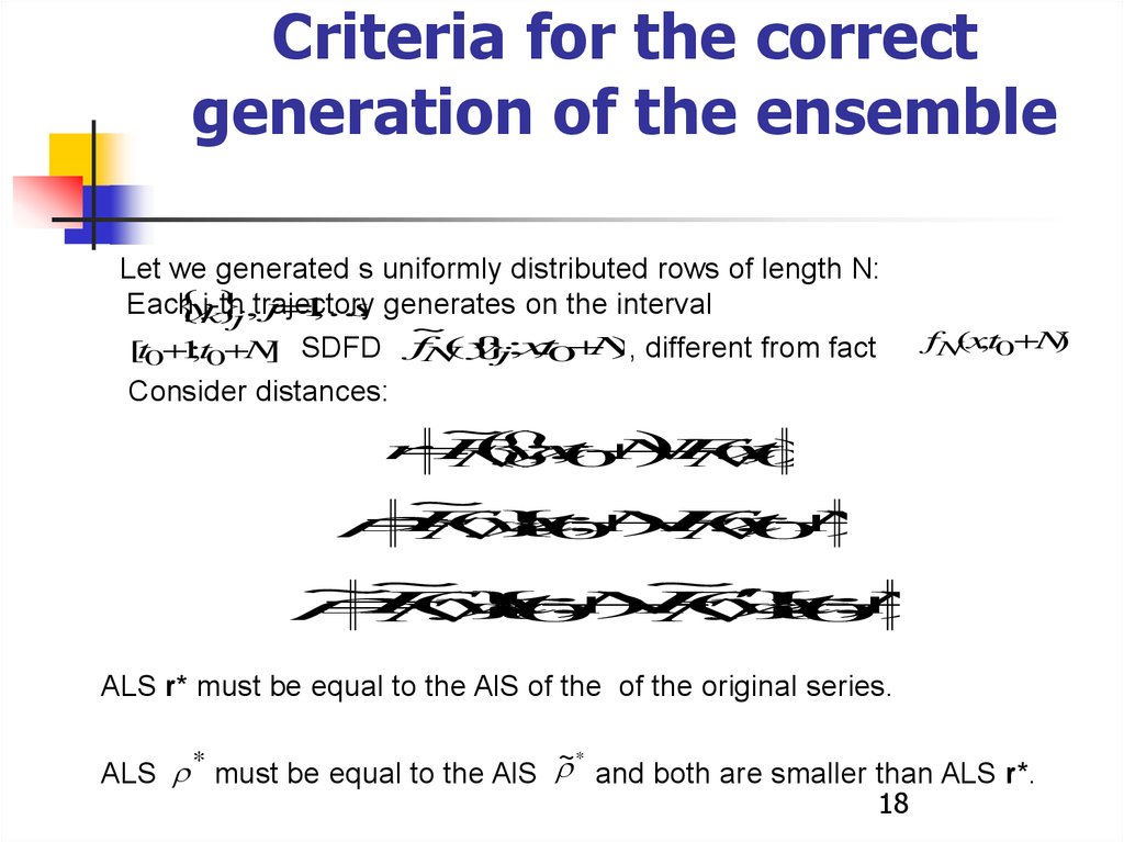
Criteria for the correctgeneration of the ensemble
Let we generated s uniformly distributed rows of length N:
Each
j-th
yk
j,trajectory
j 1
,...,
s generates on the interval
~
({
y
}
,t0
N
), different from fact
[t0 1
;t0 N] SDFD fN
j;x
Consider distances:
~
r
F
y
;
x
,
t
N
F
(
x
,
t
)
N
0
N
0
fN(x,t0 N)
~
F
({
y
};
x
,
t
N
)
F
(
x
,
t
N
)
N
0
N
0
~
~
~
F
({
y
};
x
,
t
N
)
F
({
y
};
x
,
t
N
)
N
0
N
0
ALS r* must be equal to the AlS of the of the original series.
~*
*
ALS must be equal to the AlS and both are smaller than ALS r*.
18
18.
Practical examplesExample 1 - earthquake statistics
In problems of earthquake prediction the main objects of analysis are the
regional magnitudes distribution functions
and distribution functions of time intervals between successive events.
These functions shows growth or decrease of seismic activity.
• We have studied the nonstationarity of these distributions
• We have taken a time series of earthquake magnitudes in Japan from
1916 to January 2011 according to the regional catalog JMA
(Japan Meteorological Agency)
• Gutenberg–Richter law expresses the relationship between the
magnitude and total number of earthquakes: lg(N) =a-b*M
19
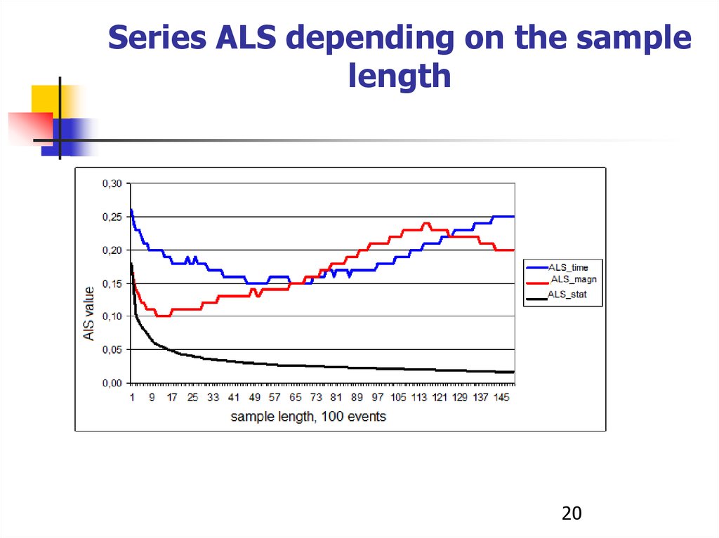
19.
Series ALS depending on the samplelength
20
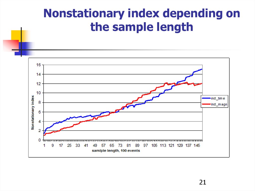
20.
Nonstationary index depending onthe sample length
21
21.
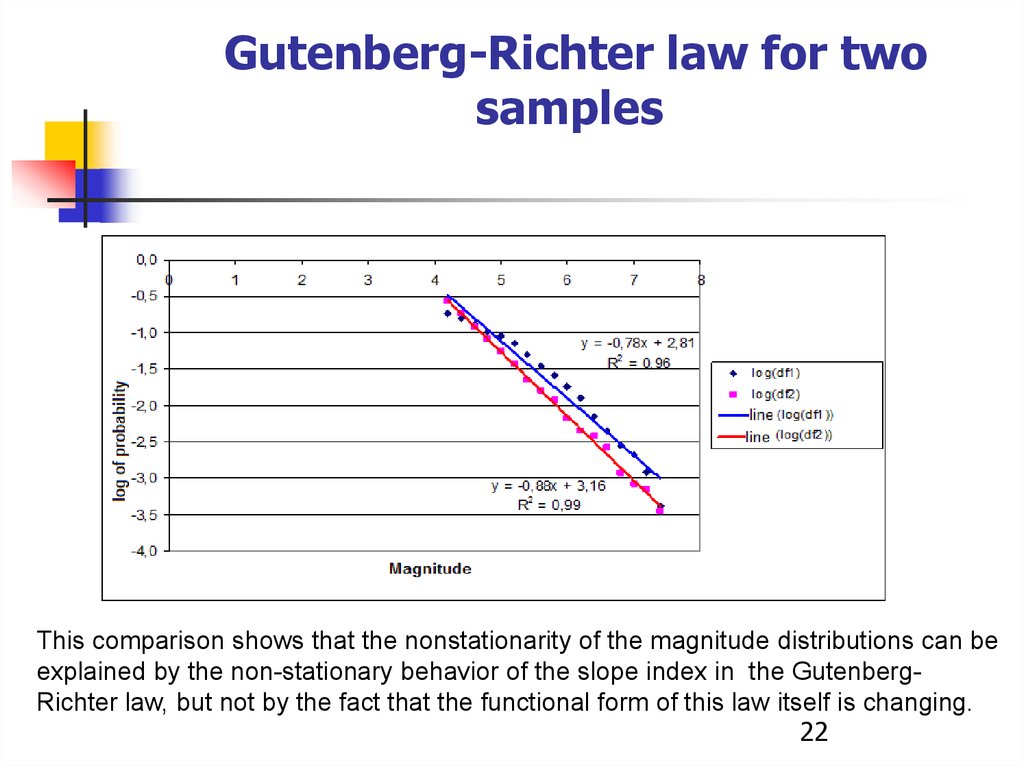
Gutenberg-Richter law for twosamples
This comparison shows that the nonstationarity of the magnitude distributions can be
explained by the non-stationary behavior of the slope index in the GutenbergRichter law, but not by the fact that the functional form of this law itself is changing.
22
22.
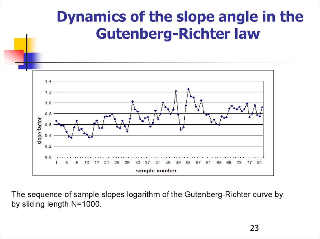
Dynamics of the slope angle in theGutenberg-Richter law
The sequence of sample slopes logarithm of the Gutenberg-Richter curve by
by sliding length N=1000.
23
23.
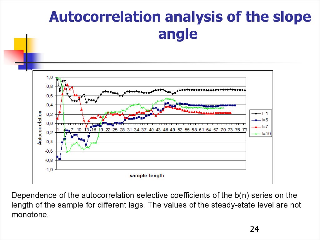
Autocorrelation analysis of the slopeangle
Dependence of the autocorrelation selective coefficients of the b(n) series on the
length of the sample for different lags. The values of the steady-state level are not
monotone.
24
24.
The values of the steady-statecoefficients of autocorrelation
depending on the lag
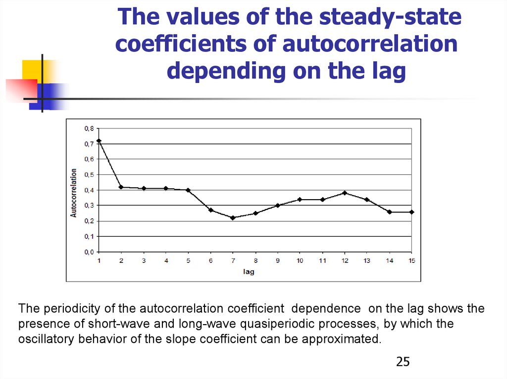
The periodicity of the autocorrelation coefficient dependence on the lag shows the
presence of short-wave and long-wave quasiperiodic processes, by which the
oscillatory behavior of the slope coefficient can be approximated.
25
25.
The model of the time series b(n)The dynamics of the values b(n) can be described by some quasiperiodic dynamical
system with additive noise.
b(n) y1 (n) y2 (n) (n)
1 n 53;
0,45 0,008n ,
y1 (n)
y1 (53) 0,008 n 53 , n 53.
0,2 0,08(n 1) ,
y 2 ( n)
y 2 (6) 0,08 n 6 ,
1 n 6;
6 n 11.
Where (n) is a series of residues, the autocorrelation of which (for any lags) does
not exceed 0.013 in absolute value, the relative mean square is 0.006, and the
distribution is approximated fairly well by a normal .
26
26.
Nonstationary distributions ofmagnitudes
it was found that the nonstationarity of the distributions
magnitude is due to the fact that the parameter in the law of the GutenbergRichter depends on time, but forms a stationary time series; this
series can be represented as a superposition of two dynamical systems with
periodic behavior and a normally distributed residue that has
low amplitude
27
27.
Earthquake statisticsresults
We analyzed the stationary level of JMA catalog of magnitude and
time intervals between events. It was shown, that these distributions are
nonstationary
and the time dependence of Gutenberg – Richter law parameter could be
represented as a superposition of two quasi-periodical dynamical systems with short
and long periods
28
28.
Example 2 - SIR statistics for analysis of 5Gnetworks
The reliability of mobile communication is estimated by the ratio of
signal power to interference at the receiving point – SIR.
l
U
SIR
N 0 , U
(
l)
l
U
li
i
1
In the static mode, the SIR is analyzed by combinatorial geometry
methods, but if the subscribers are in motion, then the SIR depends not
only on the density of the subscribers and the shape of the region, but
also on the law of motion. In many cases, the motion is stochastic and
can be represented as diffusion with drift ("customer wander"). Then the
trajectories of the receiving and transmitting devices are naturally
modeled with the help of a suitable F-P equation:
f
D
div
(
uf
)
f
t
2
29
29.
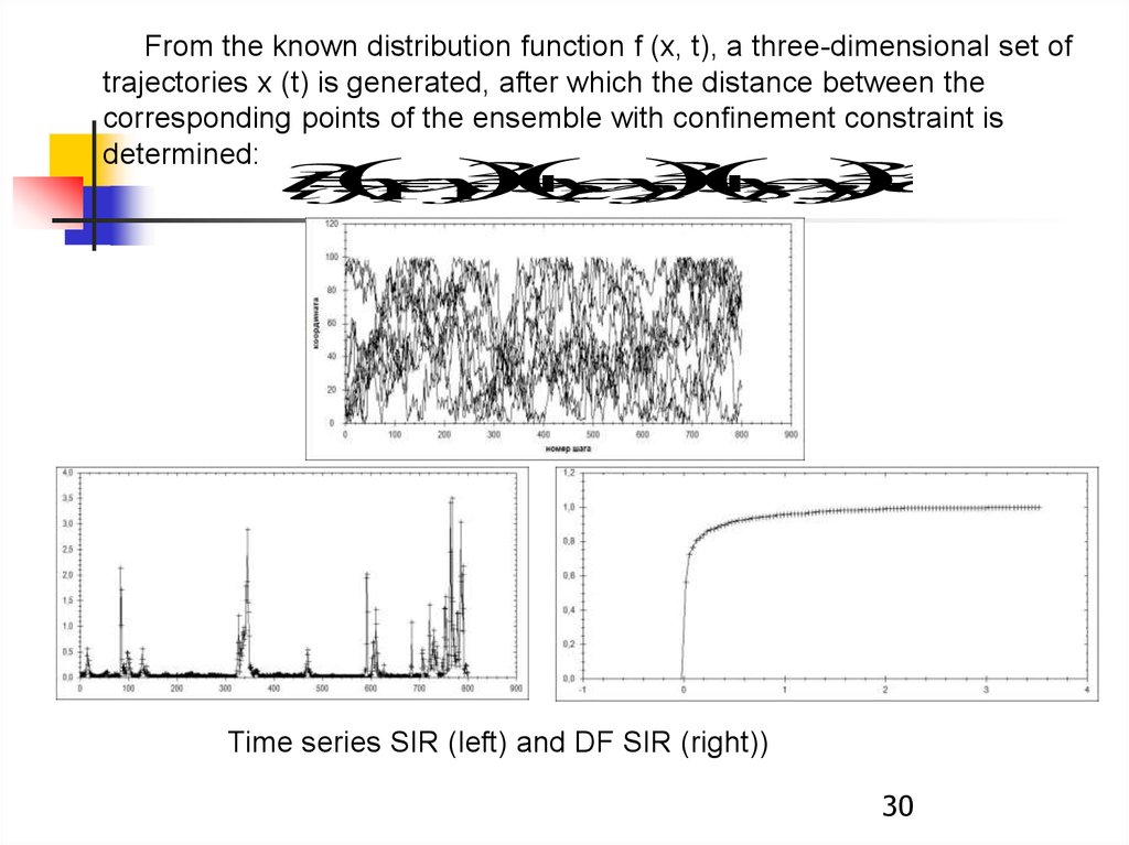
From the known distribution function f (x, t), a three-dimensional set oftrajectories x (t) is generated, after which the distance between the
corresponding points of the ensemble with confinement constraint is
determined: 2
2
2
2
2
l
x
x
x
x
x
x
a
ij
1
,
i1
,
j
2
,
i 2
,
j
3
,
i 3
,
j
Time series SIR (left) and DF SIR (right))
30
30.
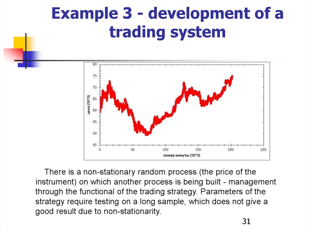
Example 3 - development of atrading system
There is a non-stationary random process (the price of the
instrument) on which another process is being built - management
through the functional of the trading strategy. Parameters of the
strategy require testing on a long sample, which does not give a
good result due to non-stationarity.
31
31.
Problems typesSelection of system parameters by historical data
Risk-management of a trading System
32
32.
Selection of system parameters byhistorical data
A small amount of historical data does not give sufficient accuracy.
However, a large volume contains in itself not current trends.
It is more efficient to generate a beam of trajectories that correspond to
evolving samples in accordance with how selective distributions of price
increases change.
33
33.
Two types of trajectiories beamgeneration
Generation by historical change of selective distribution.
Generation by forecast using Fokker-Plank equation. (Вставить формулу
горизонта пересчета, когда расхождение привысит СУС)
34
34.
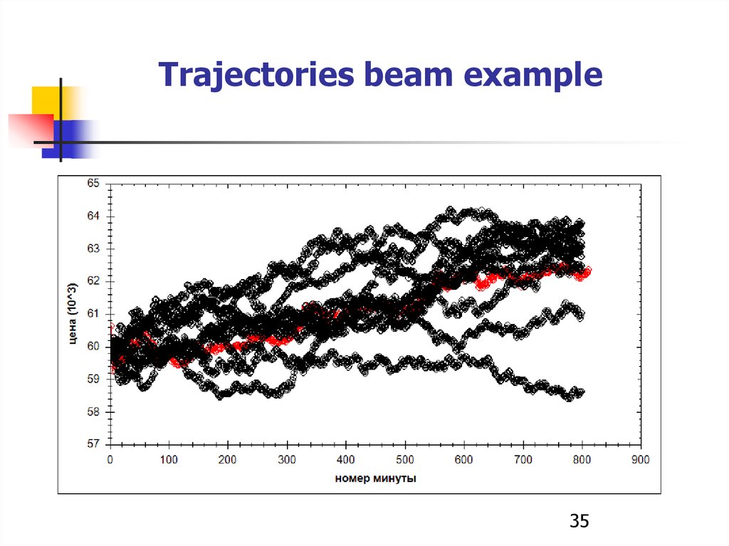
Trajectories beam example35
35.
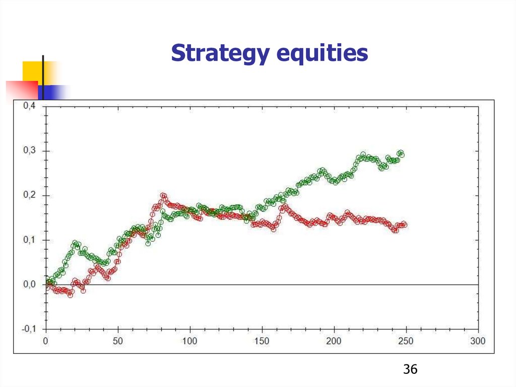
Strategy equities36
36.
ConclusionModeling of nonstationary time series has a wide practical application.
37
37.
Thank you for attention!38