Depressions and Slumps

1. Depressions and Slumps

A depression is a deep and long-lasting
recession.
Chapter 22: Depressions and Slumps
A slump is a long period of low or no growth,
longer than a typical recession, but less deep
than a depression.
Copyright © 2009 Pearson Education, Inc. Publishing as Prentice Hall • Macroeconomics, 5/e • Olivier Blanchard
1 of 43

2. 22-1 Disinflation, Deflation, and the Liquidity Trap

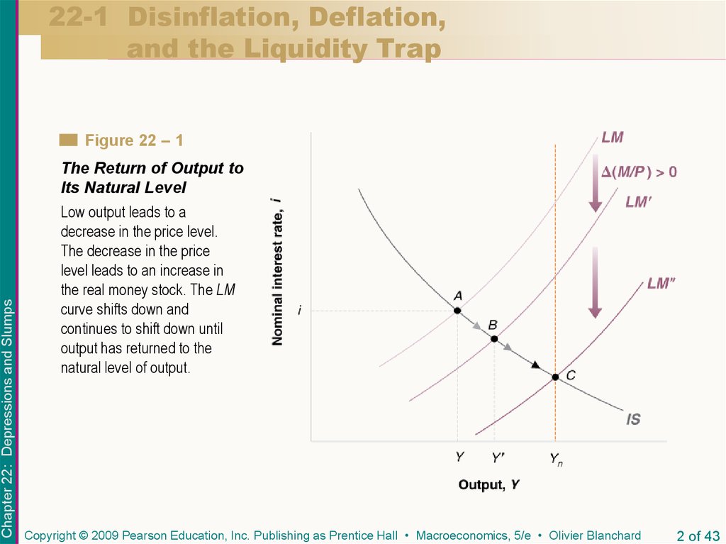
Figure 22 – 1
Chapter 22: Depressions and Slumps
The Return of Output to
Its Natural Level
Low output leads to a
decrease in the price level.
The decrease in the price
level leads to an increase in
the real money stock. The LM
curve shifts down and
continues to shift down until
output has returned to the
natural level of output.
Copyright © 2009 Pearson Education, Inc. Publishing as Prentice Hall • Macroeconomics, 5/e • Olivier Blanchard
2 of 43

3. 22-1 Disinflation, Deflation, and the Liquidity Trap

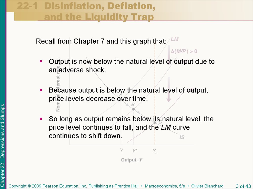
Recall from Chapter 7 and this graph that:
Output is now below the natural level of output due to
an adverse shock.
Chapter 22: Depressions and Slumps
Because output is below the natural level of output,
price levels decrease over time.
So long as output remains below its natural level, the
price level continues to fall, and the LM curve
continues to shift down.
Copyright © 2009 Pearson Education, Inc. Publishing as Prentice Hall • Macroeconomics, 5/e • Olivier Blanchard
3 of 43

4. 22-1 Disinflation, Deflation, and the Liquidity Trap

Chapters 8 and 9 presented a more realistic version of
the model.
Chapter 22: Depressions and Slumps
Suppose output is below the natural level of output –
equivalently, the unemployment rate is higher than
the natural rate of unemployment.
With the unemployment rate above the natural rate,
inflation falls over time.
As long as output is below its natural level, inflation
falls, and the LM curve continues to shift down.
Copyright © 2009 Pearson Education, Inc. Publishing as Prentice Hall • Macroeconomics, 5/e • Olivier Blanchard
4 of 43

5. 22-1 Disinflation, Deflation, and the Liquidity Trap

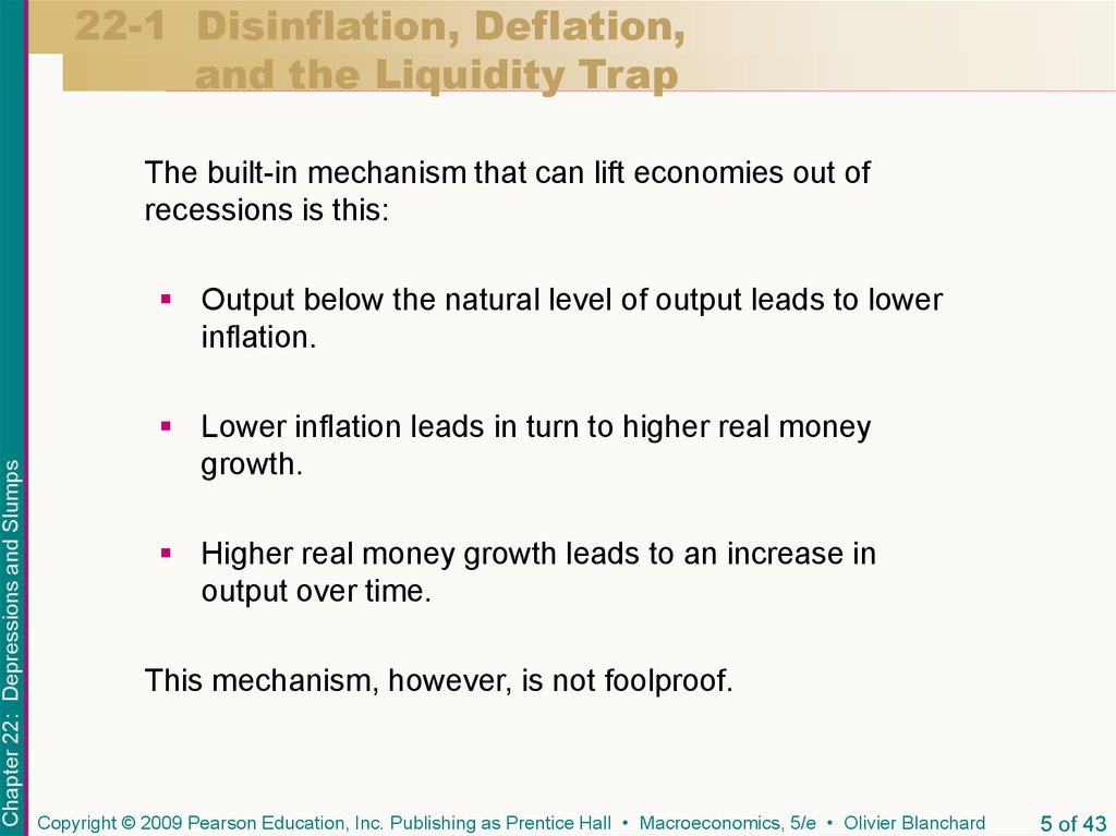
The built-in mechanism that can lift economies out of
recessions is this:
Chapter 22: Depressions and Slumps
Output below the natural level of output leads to lower
inflation.
Lower inflation leads in turn to higher real money
growth.
Higher real money growth leads to an increase in
output over time.
This mechanism, however, is not foolproof.
Copyright © 2009 Pearson Education, Inc. Publishing as Prentice Hall • Macroeconomics, 5/e • Olivier Blanchard
5 of 43

6. 22-1 Disinflation, Deflation, and the Liquidity Trap

The Nominal Interest Rate, the Real Interest Rate,
and Expected Inflation
Recall from Chapter 14 that:
Chapter 22: Depressions and Slumps
What matters for spending decisions, and thus what
enters the IS relation, is the real interest rate—the
interest rate in terms of goods.
What matters for the demand for money, and thus
enters the LM relation, is the nominal interest rate—
the interest rate in terms of dollars.
Copyright © 2009 Pearson Education, Inc. Publishing as Prentice Hall • Macroeconomics, 5/e • Olivier Blanchard
6 of 43

7. 22-1 Disinflation, Deflation, and the Liquidity Trap

The Nominal Interest Rate, the Real Interest Rate,
and Expected Inflation
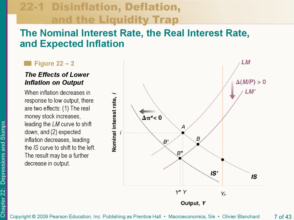
Figure 22 – 2
Chapter 22: Depressions and Slumps
The Effects of Lower
Inflation on Output
When inflation decreases in
response to low output, there
are two effects: (1) The real
money stock increases,
leading the LM curve to shift
down, and (2) expected
inflation decreases, leading
the IS curve to shift to the left.
The result may be a further
decrease in output.
Copyright © 2009 Pearson Education, Inc. Publishing as Prentice Hall • Macroeconomics, 5/e • Olivier Blanchard
7 of 43

8. 22-1 Disinflation, Deflation, and the Liquidity Trap

The Nominal Interest Rate, the Real Interest Rate,
and Expected Inflation
Chapter 22: Depressions and Slumps
Because output is below the natural level of output,
inflation falls. The decrease in inflation now has two
effects:
The first effect is to increase the real money stock
and shift the LM curve down, this shift tends to
increase output.
The second effect is for a given nominal interest
rate, the decrease in expected inflation increases
the real interest rate.
Copyright © 2009 Pearson Education, Inc. Publishing as Prentice Hall • Macroeconomics, 5/e • Olivier Blanchard
8 of 43

9. 22-1 Disinflation, Deflation, and the Liquidity Trap

The Liquidity Trap
Chapter 22: Depressions and Slumps
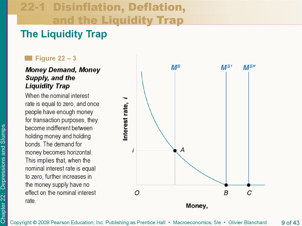
Figure 22 – 3
Money Demand, Money
Supply, and the
Liquidity Trap
When the nominal interest
rate is equal to zero, and once
people have enough money
for transaction purposes, they
become indifferent between
holding money and holding
bonds. The demand for
money becomes horizontal.
This implies that, when the
nominal interest rate is equal
to zero, further increases in
the money supply have no
effect on the nominal interest
rate.
Copyright © 2009 Pearson Education, Inc. Publishing as Prentice Hall • Macroeconomics, 5/e • Olivier Blanchard
9 of 43

10. 22-1 Disinflation, Deflation, and the Liquidity Trap

The Liquidity Trap
The demand for money is as shown in Figure 22-3.
Chapter 22: Depressions and Slumps
As the nominal interest rate decreases, people want to
hold more money.
As the nominal interest rate becomes equal to zero,
people want to hold an amount of money at least equal
to the distance OB: This is what they need for
transaction purposes.
Copyright © 2009 Pearson Education, Inc. Publishing as Prentice Hall • Macroeconomics, 5/e • Olivier Blanchard
10 of 43

11. 22-1 Disinflation, Deflation, and the Liquidity Trap

The Liquidity Trap
Now consider the effects of an increase in the money
supply:
Chapter 22: Depressions and Slumps
Starting from the equilibrium of Ms and i at point A, an
increase in the money supply leads to a decrease in the
nominal interest rate.
Now consider the case where the money supply is at
point B or C. In either case, the initial nominal interest
rate is zero, and an increase in the money supply has
no effect on the nominal interest rate at this point.
Copyright © 2009 Pearson Education, Inc. Publishing as Prentice Hall • Macroeconomics, 5/e • Olivier Blanchard
11 of 43

12. 22-1 Disinflation, Deflation, and the Liquidity Trap

The Liquidity Trap
Chapter 22: Depressions and Slumps
The liquidity trap describes a situation in which
expansionary monetary policy becomes powerless.
The increase in money falls into a liquidity trap: People
are willing to hold more money (more liquidity) at the
same nominal interest rate.
The central bank can increase “liquidity” but the
additional money is willingly held by financial investors
at an unchanged interest rate, namely, zero.
Copyright © 2009 Pearson Education, Inc. Publishing as Prentice Hall • Macroeconomics, 5/e • Olivier Blanchard
12 of 43

13. 22-1 Disinflation, Deflation, and the Liquidity Trap

The Liquidity Trap
Figure 22 – 4
Chapter 22: Depressions and Slumps
The Derivation of the LM
Curve in the Presence of
a Liquidity Trap
For low levels of output, the LM curve is a flat segment, with a nominal
interest rate equal to zero. For higher levels of output, it is upward
sloping: An increase in income leads to an increase in the nominal
interest rate.
Copyright © 2009 Pearson Education, Inc. Publishing as Prentice Hall • Macroeconomics, 5/e • Olivier Blanchard
13 of 43

14. 22-1 Disinflation, Deflation, and the Liquidity Trap

The Liquidity Trap
Chapter 22: Depressions and Slumps
To derive the LM curve, Figure 22-4(a) looks at
equilibrium in the financial markets for a given value of
the real money stock and draws three money demand
curves, each corresponding to a different level of
income:
The combination of income, Y, and nominal
interest rate, i, gives us the first point on the LM
curve, point A in Figure 22-4(b).
Lower income means fewer transactions, and,
therefore, a lower demand for money at any
interest rate. This combination of income, Y’, and
nominal interest rate, i’, gives us the second point
on the LM curve, point A’ in Figure 22-4(b).
Copyright © 2009 Pearson Education, Inc. Publishing as Prentice Hall • Macroeconomics, 5/e • Olivier Blanchard
14 of 43

15. 22-1 Disinflation, Deflation, and the Liquidity Trap

The Liquidity Trap
Chapter 22: Depressions and Slumps
The equilibrium is given by point A” in Figure 224(a), with nominal interest rate equal to zero.
Point A” in Figure 22-4(b) corresponds to A” in
Figure 22-4(a).
The intersection between the money supply curve
and the money demand curve takes place on the
horizontal portion of the money demand curve.
The equilibrium remains at A”, and the nominal
interest rate remains equal to zero.
Copyright © 2009 Pearson Education, Inc. Publishing as Prentice Hall • Macroeconomics, 5/e • Olivier Blanchard
15 of 43

16. 22-1 Disinflation, Deflation, and the Liquidity Trap

The Liquidity Trap
Figure 22 – 5
Chapter 22: Depressions and Slumps
The IS–LM Model and
the Liquidity Trap
In the presence of a liquidity
trap, there is a limit to how
much monetary policy can
increase output. Monetary
policy may not be able to
increase output back to its
natural level.
Copyright © 2009 Pearson Education, Inc. Publishing as Prentice Hall • Macroeconomics, 5/e • Olivier Blanchard
16 of 43

17. 22-1 Disinflation, Deflation, and the Liquidity Trap

Putting Things Together: The Liquidity
Trap and Deflation
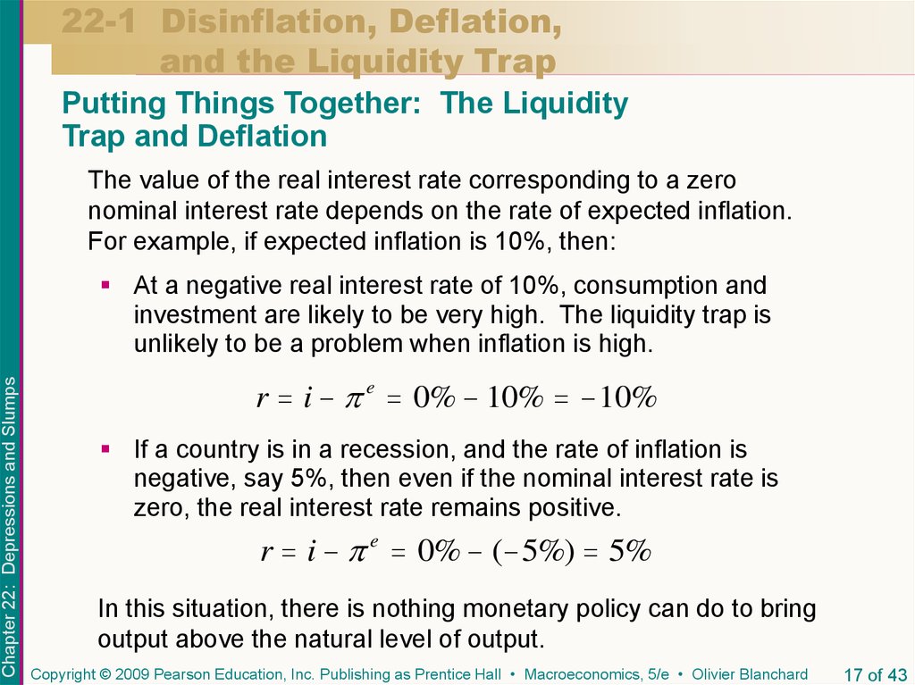
The value of the real interest rate corresponding to a zero
nominal interest rate depends on the rate of expected inflation.
For example, if expected inflation is 10%, then:
Chapter 22: Depressions and Slumps
At a negative real interest rate of 10%, consumption and
investment are likely to be very high. The liquidity trap is
unlikely to be a problem when inflation is high.
r i e 0% 10% 10%
If a country is in a recession, and the rate of inflation is
negative, say 5%, then even if the nominal interest rate is
zero, the real interest rate remains positive.
r i e 0% ( 5%) 5%
In this situation, there is nothing monetary policy can do to bring
output above the natural level of output.
Copyright © 2009 Pearson Education, Inc. Publishing as Prentice Hall • Macroeconomics, 5/e • Olivier Blanchard
17 of 43

18. 22-1 Disinflation, Deflation, and the Liquidity Trap

Putting Things Together: The Liquidity
Trap and Deflation
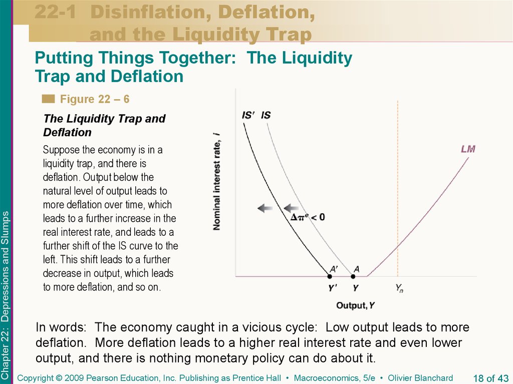
Figure 22 – 6
Chapter 22: Depressions and Slumps
The Liquidity Trap and
Deflation
Suppose the economy is in a
liquidity trap, and there is
deflation. Output below the
natural level of output leads to
more deflation over time, which
leads to a further increase in the
real interest rate, and leads to a
further shift of the IS curve to the
left. This shift leads to a further
decrease in output, which leads
to more deflation, and so on.
In words: The economy caught in a vicious cycle: Low output leads to more
deflation. More deflation leads to a higher real interest rate and even lower
output, and there is nothing monetary policy can do about it.
Copyright © 2009 Pearson Education, Inc. Publishing as Prentice Hall • Macroeconomics, 5/e • Olivier Blanchard
18 of 43

19. 22-2 The Great Depression

Figure 22 – 7
The U.S. Unemployment
Rate, 1920 to 1950
Chapter 22: Depressions and Slumps
The Great Depression was
characterized by a sharp
increase in unemployment,
followed by a slow decline.
Copyright © 2009 Pearson Education, Inc. Publishing as Prentice Hall • Macroeconomics, 5/e • Olivier Blanchard
19 of 43

20. 22-2 The Great Depression

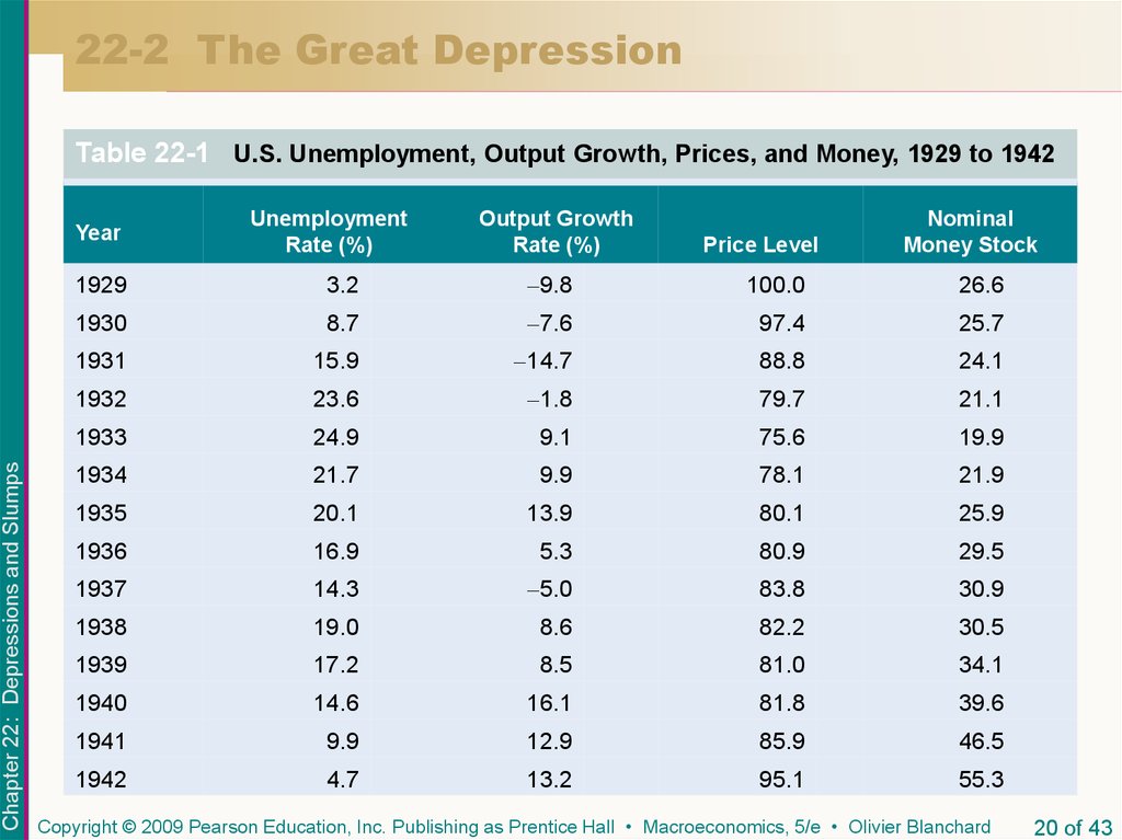
Table 22-1 U.S. Unemployment, Output Growth, Prices, and Money, 1929 to 1942
Chapter 22: Depressions and Slumps
Year
Unemployment
Rate (%)
Output Growth
Rate (%)
Price Level
Nominal
Money Stock
1929
3.2
9.8
100.0
26.6
1930
8.7
7.6
97.4
25.7
1931
15.9
14.7
88.8
24.1
1932
23.6
1.8
79.7
21.1
1933
24.9
9.1
75.6
19.9
1934
21.7
9.9
78.1
21.9
1935
20.1
13.9
80.1
25.9
1936
16.9
5.3
80.9
29.5
1937
14.3
5.0
83.8
30.9
1938
19.0
8.6
82.2
30.5
1939
17.2
8.5
81.0
34.1
1940
14.6
16.1
81.8
39.6
1941
9.9
12.9
85.9
46.5
1942
4.7
13.2
95.1
55.3
Copyright © 2009 Pearson Education, Inc. Publishing as Prentice Hall • Macroeconomics, 5/e • Olivier Blanchard
20 of 43

21. 22-2 The Great Depression

Focusing only on unemployment and output for the
moment, two facts emerge from the table:
How sharply and how much output declined at the start
of the depression.
Chapter 22: Depressions and Slumps
How long it then took for unemployment to recover.
The Initial Fall in Spending
A recession had actually started before the stock market
crash of October, 1929. The crash, however, was
important.
The stock market crash not only decreased consumers’
wealth, it also increased their uncertainty about the future.
Copyright © 2009 Pearson Education, Inc. Publishing as Prentice Hall • Macroeconomics, 5/e • Olivier Blanchard
21 of 43

22. 22-2 The Great Depression

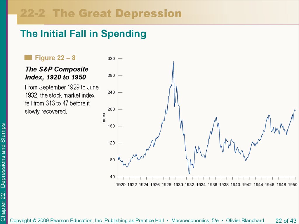
The Initial Fall in Spending
Figure 22 – 8
The S&P Composite
Index, 1920 to 1950
Chapter 22: Depressions and Slumps
From September 1929 to June
1932, the stock market index
fell from 313 to 47 before it
slowly recovered.
Copyright © 2009 Pearson Education, Inc. Publishing as Prentice Hall • Macroeconomics, 5/e • Olivier Blanchard
22 of 43

23. 22-2 The Great Depression

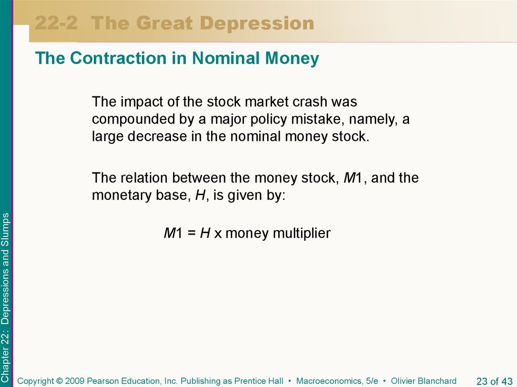
The Contraction in Nominal Money
The impact of the stock market crash was
compounded by a major policy mistake, namely, a
large decrease in the nominal money stock.
Chapter 22: Depressions and Slumps
The relation between the money stock, M1, and the
monetary base, H, is given by:
M1 = H x money multiplier
Copyright © 2009 Pearson Education, Inc. Publishing as Prentice Hall • Macroeconomics, 5/e • Olivier Blanchard
23 of 43

24. 22-2 The Great Depression

The Contraction in Nominal Money
Chapter 22: Depressions and Slumps
Table 22-2 Money, Nominal and Real, 1929 to 1933
Year
Nominal Money
Stock, M1
Monetary
Base, H
Money
Multiplier, M1/H
Real Money
Stock, M1/P
1929
26.6
7.1
3.7
26.4
1930
25.7
6.9
3.7
26.0
1931
24.1
7.3
3.3
26.5
1932
21.1
7.8
2.7
25.8
1933
19.4
8.2
2.4
25.6
During the Great Depression, the decrease in the money supply
came from a decrease in the money multiplier (M1/H), as
people shifted their money from checkable deposits to currency.
The decrease in the money supply was roughly proportional to
the decrease in the price level. Consequently, the LM curve
remained roughly unchanged.
Copyright © 2009 Pearson Education, Inc. Publishing as Prentice Hall • Macroeconomics, 5/e • Olivier Blanchard
24 of 43

25. 22-2 The Great Depression

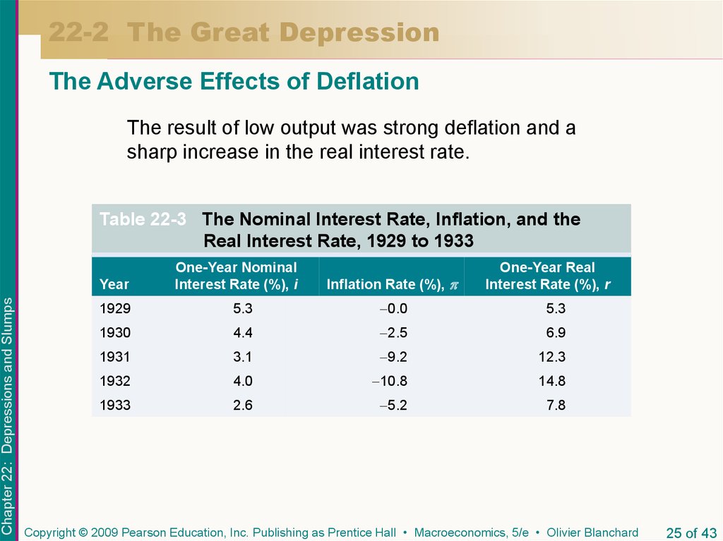
The Adverse Effects of Deflation
The result of low output was strong deflation and a
sharp increase in the real interest rate.
Table 22-3 The Nominal Interest Rate, Inflation, and the
Real Interest Rate, 1929 to 1933
Chapter 22: Depressions and Slumps
Year
One-Year Nominal
Interest Rate (%), i
Inflation Rate (%),
One-Year Real
Interest Rate (%), r
1929
5.3
0.0
5.3
1930
4.4
2.5
6.9
1931
3.1
9.2
12.3
1932
4.0
10.8
14.8
1933
2.6
5.2
7.8
Copyright © 2009 Pearson Education, Inc. Publishing as Prentice Hall • Macroeconomics, 5/e • Olivier Blanchard
25 of 43

26. 22-2 The Great Depression

The Recovery
Monetary policy played an important role in the recovery. From
1933 to 1941, the nominal money stock increased by 140% and
the real money stock by 100%. These increases were due to
increases in the monetary base, not the money multiplier.
Chapter 22: Depressions and Slumps
Other factors that played an important role were:
The New Deal—a set of programs implemented by the
Roosevelt administration.
The creation of the Federal Deposit Insurance Corporation
(FDIC).
Other programs administered by the National Recovery
Administration (NRA).
Copyright © 2009 Pearson Education, Inc. Publishing as Prentice Hall • Macroeconomics, 5/e • Olivier Blanchard
26 of 43

27. 22-2 The Great Depression

The Recovery
The puzzle is why deflation ended in 1933.
Chapter 22: Depressions and Slumps
One proximate cause may be the set of measures taken by
the Roosevelt administration such as establishing the
National Industrial Recovery Act (NIRA) of 1933.
Another factor may be that while unemployment was still
high, output growth was high as well.
Another factor may be the perception of a “regime change”
associated with the election of Roosevelt.
Copyright © 2009 Pearson Education, Inc. Publishing as Prentice Hall • Macroeconomics, 5/e • Olivier Blanchard
27 of 43

28. 22-3 The Japanese Slump

The robust growth that Japan had experienced since the
end of World War II came to an end in the early 1990s.
Chapter 22: Depressions and Slumps
Since 1992, the economy has suffered from a long period
of low growth—what is called the Japanese slump.
Low growth has led to a steady increase in unemployment,
and a steady decrease in the inflation rate over time.
Copyright © 2009 Pearson Education, Inc. Publishing as Prentice Hall • Macroeconomics, 5/e • Olivier Blanchard
28 of 43

29. 22-3 The Japanese Slump

Figure 22 – 9
The Japanese Slump:
Output Growth since
1990 (percent)
Chapter 22: Depressions and Slumps
From 1992 to 2002, average
GDP growth in Japan was
less than 1%.
Copyright © 2009 Pearson Education, Inc. Publishing as Prentice Hall • Macroeconomics, 5/e • Olivier Blanchard
29 of 43

30. 22-3 The Japanese Slump

Figure 22 – 10
Unemployment and
Inflation in Japan since
1990 (percent)
Chapter 22: Depressions and Slumps
Low growth in output has
led to an increase in
unemployment. Inflation has
turned into deflation.
Copyright © 2009 Pearson Education, Inc. Publishing as Prentice Hall • Macroeconomics, 5/e • Olivier Blanchard
30 of 43

31. 22-3 The Japanese Slump

Chapter 22: Depressions and Slumps
Table 22-4 GDP, Consumption, and Investment Growth, Japan, 1988-1993
Year
GDP (%)
Consumption (%)
Investment (%)
1988
6.5
5.1
15.5
1989
5.3
4.7
15.0
1990
5.2
4.6
10.1
1991
3.4
2.9
4.3
1992
1.0
2.6
7.1
1993
0.2
1.4
10.3
The numbers in Table 22-4 raise an obvious set of questions:
What triggered Japan’s slump? Why did it last so long? Were
monetary and fiscal policies misused, or did they fail? What are
the factors behind the current recovery?
Copyright © 2009 Pearson Education, Inc. Publishing as Prentice Hall • Macroeconomics, 5/e • Olivier Blanchard
31 of 43

32. 22-3 The Japanese Slump

The Rise and Fall of the Nikkei
There are two reasons for the increase in a stock price:
Chapter 22: Depressions and Slumps
A change in the fundamental value of the stock
price, which depends on the expected present value
of future dividends.
A speculative bubble: Investors buy at a higher
price simply because they expect the price to go
even higher in the future.
Copyright © 2009 Pearson Education, Inc. Publishing as Prentice Hall • Macroeconomics, 5/e • Olivier Blanchard
32 of 43

33. 22-3 The Japanese Slump

The Rise and Fall of the Nikkei
Figure 22 – 11
Chapter 22: Depressions and Slumps
Stock Prices and
Dividends in Japan
since 1980
The increase in stock prices
in the 1980s and the
subsequent decrease were
not associated with a
parallel movement in
dividends.
Copyright © 2009 Pearson Education, Inc. Publishing as Prentice Hall • Macroeconomics, 5/e • Olivier Blanchard
33 of 43

34. 22-3 The Japanese Slump

The Rise and Fall of the Nikkei
Chapter 22: Depressions and Slumps
The fact that dividends remained flat while stock prices
increased strongly suggests that a large bubble existed in
the Nikkei.
The rapid fall in stock prices had a major impact on
spending—consumption was less affected, but investment
collapsed.
Copyright © 2009 Pearson Education, Inc. Publishing as Prentice Hall • Macroeconomics, 5/e • Olivier Blanchard
34 of 43

35. 22-3 The Japanese Slump

The Failure of Monetary and Fiscal Policy
Chapter 22: Depressions and Slumps
Figure 22 – 12
The Nominal Interest
Rate and the Real
Interest Rate in Japan
since 1990
Japan has been in a liquidity
trap since the mid-1990s:
The nominal interest rate
has been close to zero, and
the inflation rate has been
negative. Even at a zero
nominal interest rate, the
real interest rate has been
positive.
Copyright © 2009 Pearson Education, Inc. Publishing as Prentice Hall • Macroeconomics, 5/e • Olivier Blanchard
35 of 43

36. 22-3 The Japanese Slump

The Failure of Monetary and Fiscal Policy
Chapter 22: Depressions and Slumps
Monetary policy was used, but it was used too late,
and when it was used, if faced the twin problems of
the liquidity trap and deflation.
The Bank of Japan (BoJ) cut the nominal interest rate,
but it did so slowly, and the cumulative effect of low
growth was such that inflation had turned to deflation.
As a result, the real interest rate was higher than the
nominal interest rate.
Copyright © 2009 Pearson Education, Inc. Publishing as Prentice Hall • Macroeconomics, 5/e • Olivier Blanchard
36 of 43

37. 22-3 The Japanese Slump

The Failure of Monetary and Fiscal Policy
Chapter 22: Depressions and Slumps
Fiscal policy was used as well. Taxes decreased at
the start of the slump, and there was a steady
increase in government spending throughout the
decade.
Fiscal policy helped, but it was not enough to increase
spending and output.
Copyright © 2009 Pearson Education, Inc. Publishing as Prentice Hall • Macroeconomics, 5/e • Olivier Blanchard
37 of 43

38. 22-3 The Japanese Slump

The Failure of Monetary and Fiscal Policy
Chapter 22: Depressions and Slumps
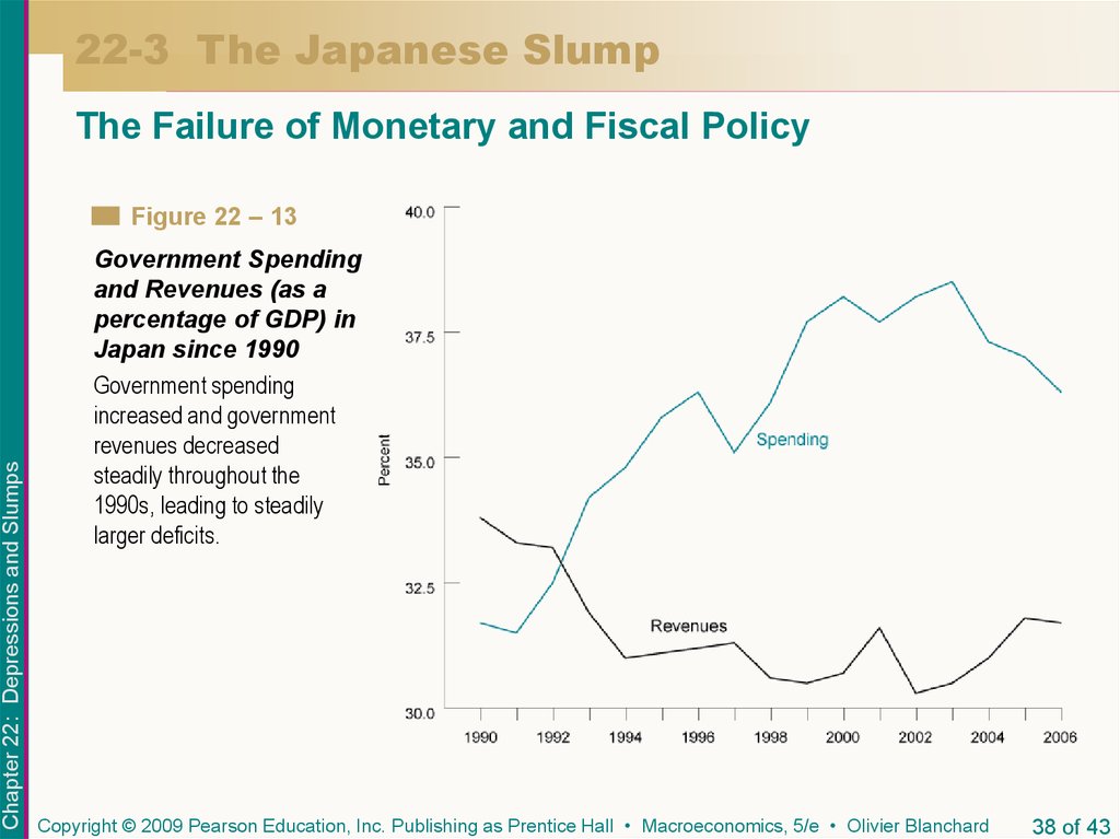
Figure 22 – 13
Government Spending
and Revenues (as a
percentage of GDP) in
Japan since 1990
Government spending
increased and government
revenues decreased
steadily throughout the
1990s, leading to steadily
larger deficits.
Copyright © 2009 Pearson Education, Inc. Publishing as Prentice Hall • Macroeconomics, 5/e • Olivier Blanchard
38 of 43

39. 22-3 The Japanese Slump

The Japanese Recovery
Output growth has been higher since 2003, and most
economists cautiously predict that the recovery will
continue. This raises the last set of questions. What
are the factors behind the current recovery?
Chapter 22: Depressions and Slumps
There appear to be two main factors.
Copyright © 2009 Pearson Education, Inc. Publishing as Prentice Hall • Macroeconomics, 5/e • Olivier Blanchard
39 of 43

40. 22-3 The Japanese Slump

The Japanese Recovery
A Regime Change in Monetary Policy
Chapter 22: Depressions and Slumps
It is suggested that even if the nominal interest rate is
already equal to zero and thus cannot be reduced further,
the central bank might still be able to lower the real interest
rate by affecting inflation expectations.
The Cleanup of the Banking System
It became clear in the 1990s that the banking system in
Japan was in trouble. Since 2002, the government has put
increasing pressure on banks to reduce bad loans, and
banks, in turn, have put increasing pressure on bad firms to
restructure or close.
Copyright © 2009 Pearson Education, Inc. Publishing as Prentice Hall • Macroeconomics, 5/e • Olivier Blanchard
40 of 43

41.

The Japanese Banking Problem
Chapter 22: Depressions and Slumps
Like the Great Depression in the U.S., the sharp
decrease in output growth in Japan in the early 1990s
left many firms unable to repay their bank loans.
Figure 1 The Bank’s Balance Sheet
Copyright © 2009 Pearson Education, Inc. Publishing as Prentice Hall • Macroeconomics, 5/e • Olivier Blanchard
41 of 43

42. Key Terms

Chapter 22: Depressions and Slumps
depression
slump
liquidity trap
New Deal
National Recovery Administration (NRA)
National Industrial Recovery Act (NIRA)
Copyright © 2009 Pearson Education, Inc. Publishing as Prentice Hall • Macroeconomics, 5/e • Olivier Blanchard
42 of 43