Production

1. Chapter 6

Production

2. Topics to be Discussed

The Technology of Production
Production with One Variable Input
(Labor)
Isoquants
Production with Two Variable Inputs
Returns to Scale
©2005 Pearson Education, Inc.
Chapter 6
2

3. Introduction

Our study of consumer behavior was
broken down into 3 steps:
Describing consumer preferences
Consumers face budget constraints
Consumers choose to maximize utility
Production decisions of a firm are similar
to consumer decisions
Can also be broken down into three steps
©2005 Pearson Education, Inc.
Chapter 6
3

4. Production Decisions of a Firm

1. Production Technology
Describe how inputs can be transformed
into outputs
Inputs: land, labor, capital and raw materials
Outputs: cars, desks, books, etc.
Firms can produce different amounts of
outputs using different combinations of
inputs
©2005 Pearson Education, Inc.
Chapter 6
4

5. Production Decisions of a Firm

2. Cost Constraints
Firms must consider prices of labor, capital
and other inputs
Firms want to minimize total production
costs partly determined by input prices
As consumers must consider budget
constraints, firms must be concerned about
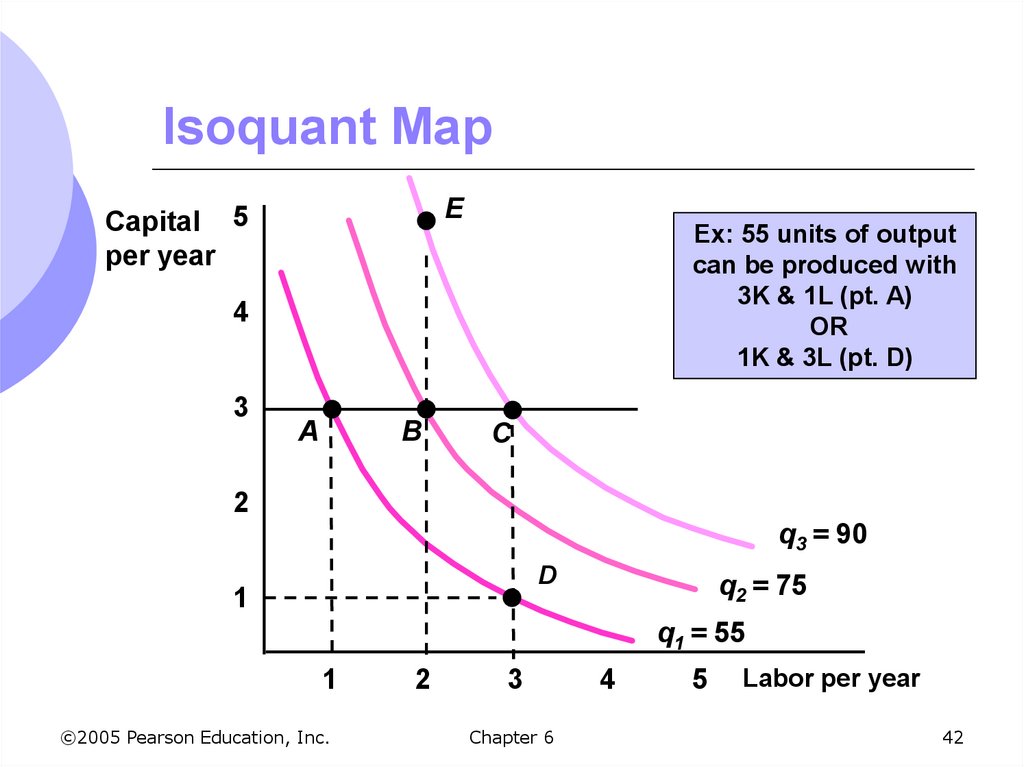
costs of production
©2005 Pearson Education, Inc.
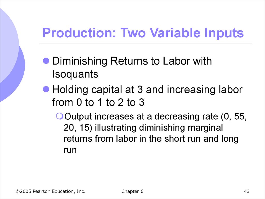
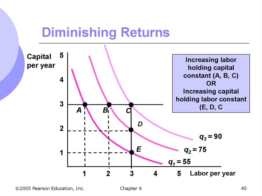
Chapter 6
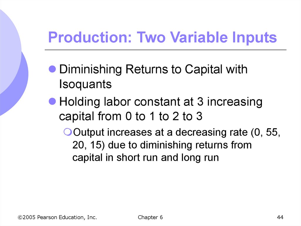
5

6. Production Decisions of a Firm

3. Input Choices
Given input prices and production
technology, the firm must choose how much
of each input to use in producing output
Given prices of different inputs, the firm
may choose different combinations of inputs
to minimize costs
If labor is cheap, firm may choose to produce
with more labor and less capital
©2005 Pearson Education, Inc.
Chapter 6
6

7. Production Decisions of a Firm

If a firm is a cost minimizer, we can also
study
How total costs of production vary with
output
How the firm chooses the quantity to
maximize its profits
We can represent the firm’s production
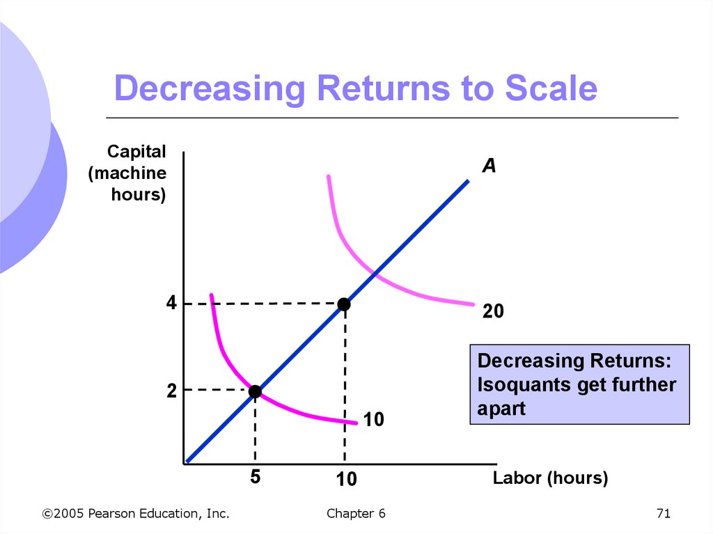
technology in the form of a production
function
©2005 Pearson Education, Inc.
Chapter 6
7

8. The Technology of Production

Production Function:
Indicates the highest output (q) that a firm
can produce for every specified combination
of inputs
For simplicity, we will consider only labor (L)
and capital (K)
Shows what is technically feasible when the
firm operates efficiently
©2005 Pearson Education, Inc.
Chapter 6
8

9. The Technology of Production

The production function for two inputs:
q = F(K,L)
Output (q) is a function of capital (K) and
labor (L)
The production function is true for a given
technology
If technology increases, more output can be
produced for a given level of inputs
©2005 Pearson Education, Inc.
Chapter 6
9

10. The Technology of Production

Short Run versus Long Run
It takes time for a firm to adjust production
from one set of inputs to another
Firms must consider not only what inputs can
be varied but over what period of time that
can occur
We must distinguish between long run and
short run
©2005 Pearson Education, Inc.
Chapter 6
10

11. The Technology of Production

Short Run
Period of time in which quantities of one or
more production factors cannot be changed
These inputs are called fixed inputs
Long Run
Amount of time needed to make all
production inputs variable
Short run and long run are not time
specific
©2005 Pearson Education, Inc.
Chapter 6
11

12. Production: One Variable Input

We will begin looking at the short run
when only one input can be varied
We assume capital is fixed and labor is
variable
Output can only be increased by increasing
labor
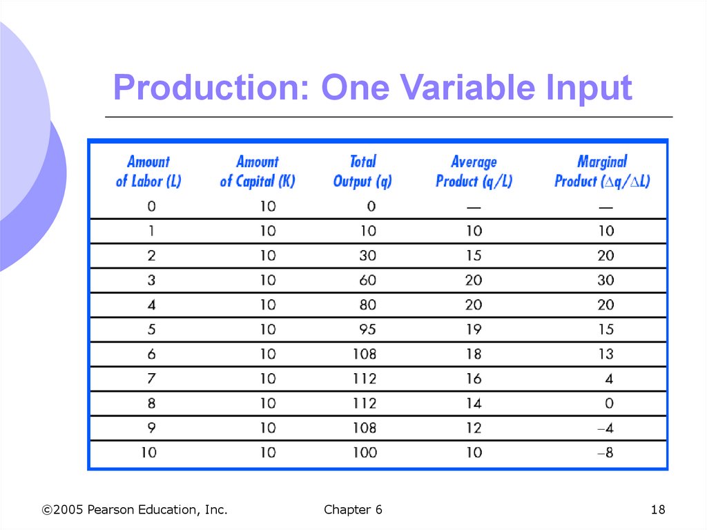
Must know how output changes as the
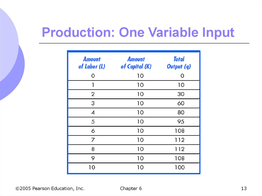
amount of labor is changed (Table 6.1)
©2005 Pearson Education, Inc.
Chapter 6
12

13. Production: One Variable Input

©2005 Pearson Education, Inc.
Chapter 6
13

14. Production: One Variable Input

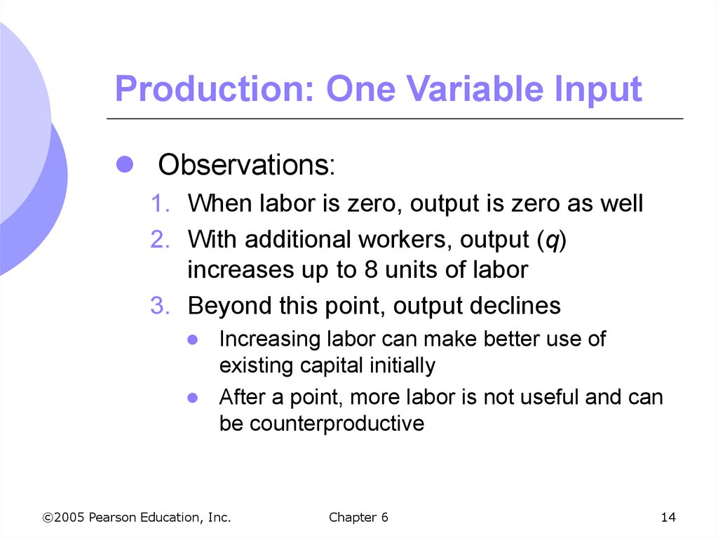
Observations:
1. When labor is zero, output is zero as well
2. With additional workers, output (q)
increases up to 8 units of labor
3. Beyond this point, output declines
Increasing labor can make better use of
existing capital initially
After a point, more labor is not useful and can
be counterproductive
©2005 Pearson Education, Inc.
Chapter 6
14

15. Production: One Variable Input

Firms make decisions based on the
benefits and costs of production
Sometimes useful to look at benefits and
costs on an incremental basis
How much more can be produced when at
incremental units of an input?
Sometimes useful to make comparison
on an average basis
©2005 Pearson Education, Inc.
Chapter 6
15

16. Production: One Variable Input

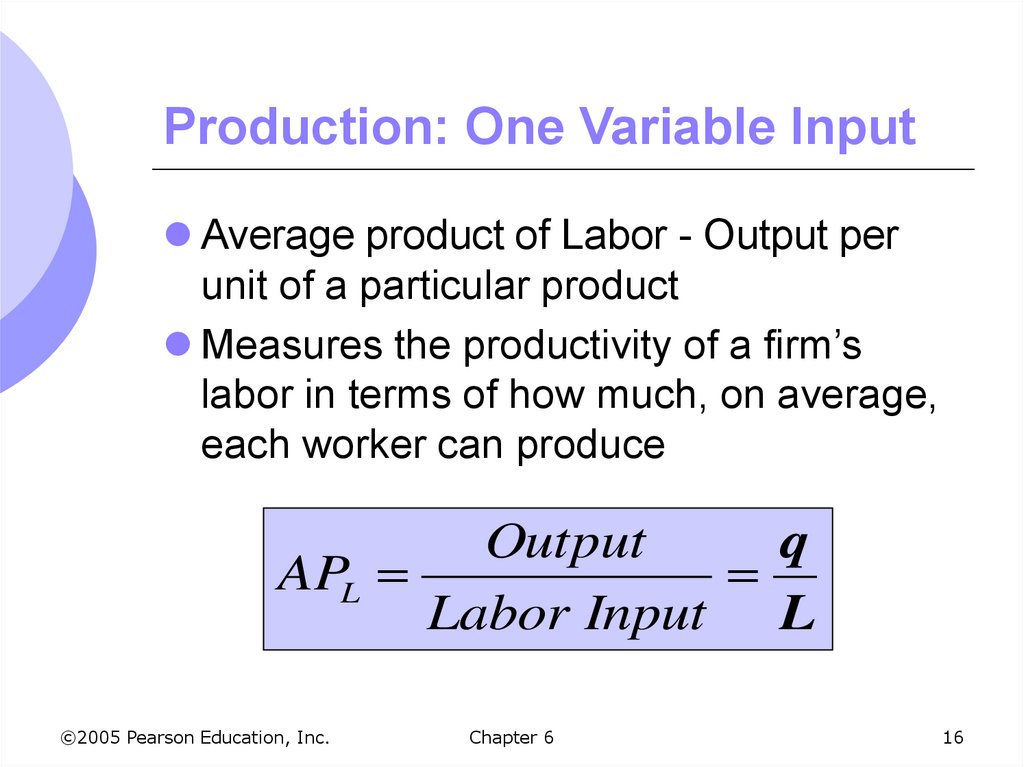
Average product of Labor - Output per
unit of a particular product
Measures the productivity of a firm’s
labor in terms of how much, on average,
each worker can produce
Output
q
APL
Labor Input L
©2005 Pearson Education, Inc.
Chapter 6
16

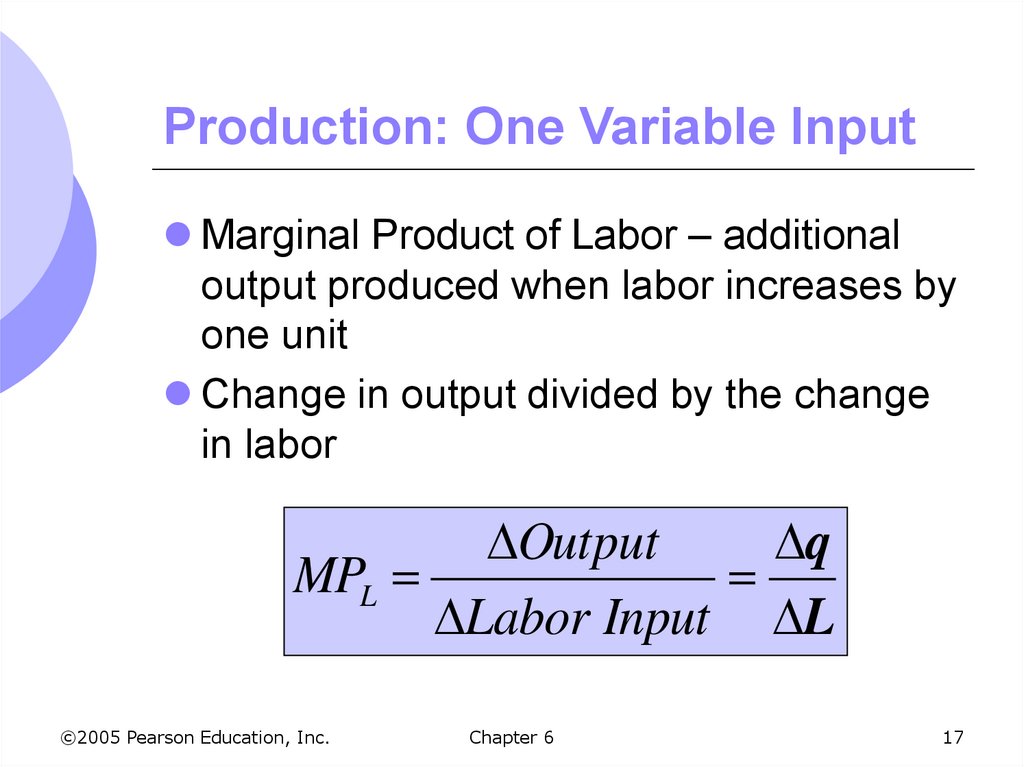
17. Production: One Variable Input

Marginal Product of Labor – additional
output produced when labor increases by
one unit
Change in output divided by the change
in labor
Output
q
MPL
Labor Input L
©2005 Pearson Education, Inc.
Chapter 6
17

18. Production: One Variable Input

©2005 Pearson Education, Inc.
Chapter 6
18

19. Production: One Variable Input

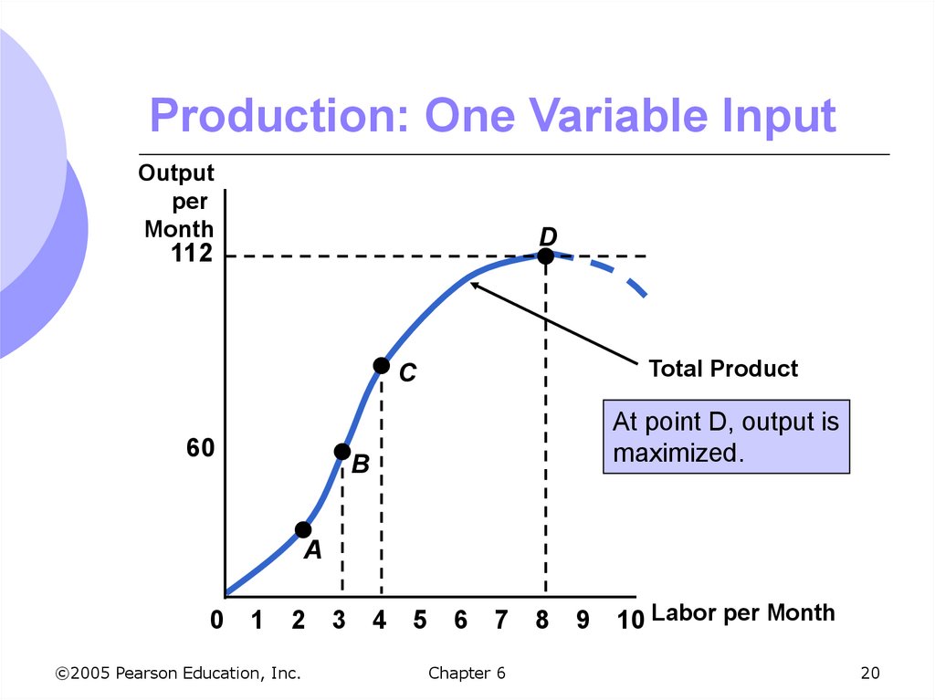
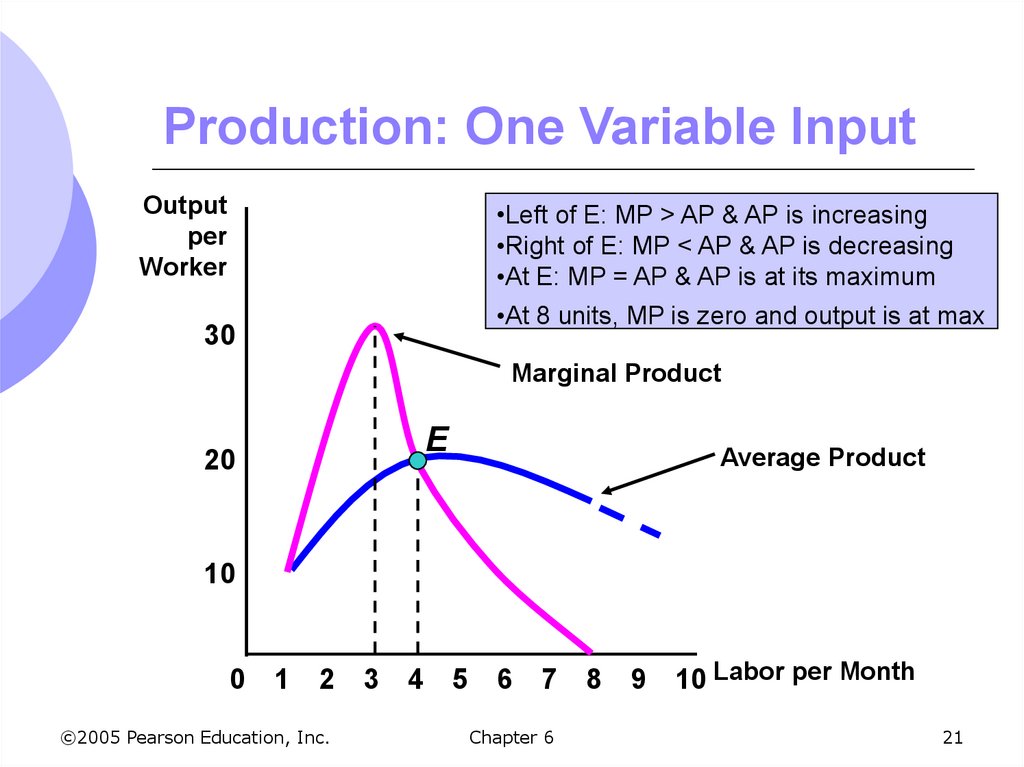
We can graph the information in Table
6.1 to show
How output varies with changes in labor
Output is maximized at 112 units
Average and Marginal Products
Marginal Product is positive as long as total
output is increasing
Marginal Product crosses Average Product at its
maximum
©2005 Pearson Education, Inc.
Chapter 6
19

20. Production: One Variable Input

Output
per
Month
D
112
Total Product
C
60
At point D, output is
maximized.
B
A
0 1
2 3
©2005 Pearson Education, Inc.
4
5 6
7 8
Chapter 6
9
10 Labor per Month
20

21. Production: One Variable Input

Output
per
Worker
•Left of E: MP > AP & AP is increasing
•Right of E: MP < AP & AP is decreasing
•At E: MP = AP & AP is at its maximum
•At 8 units, MP is zero and output is at max
30
Marginal Product
E
20
Average Product
10
0 1
2 3
©2005 Pearson Education, Inc.
4
5 6
7 8
Chapter 6
9
10 Labor per Month
21

22. Marginal and Average Product

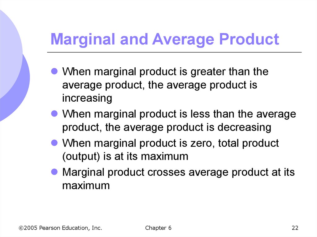
When marginal product is greater than the
average product, the average product is
increasing
When marginal product is less than the average
product, the average product is decreasing
When marginal product is zero, total product
(output) is at its maximum
Marginal product crosses average product at its
maximum
©2005 Pearson Education, Inc.
Chapter 6
22

23. Product Curves

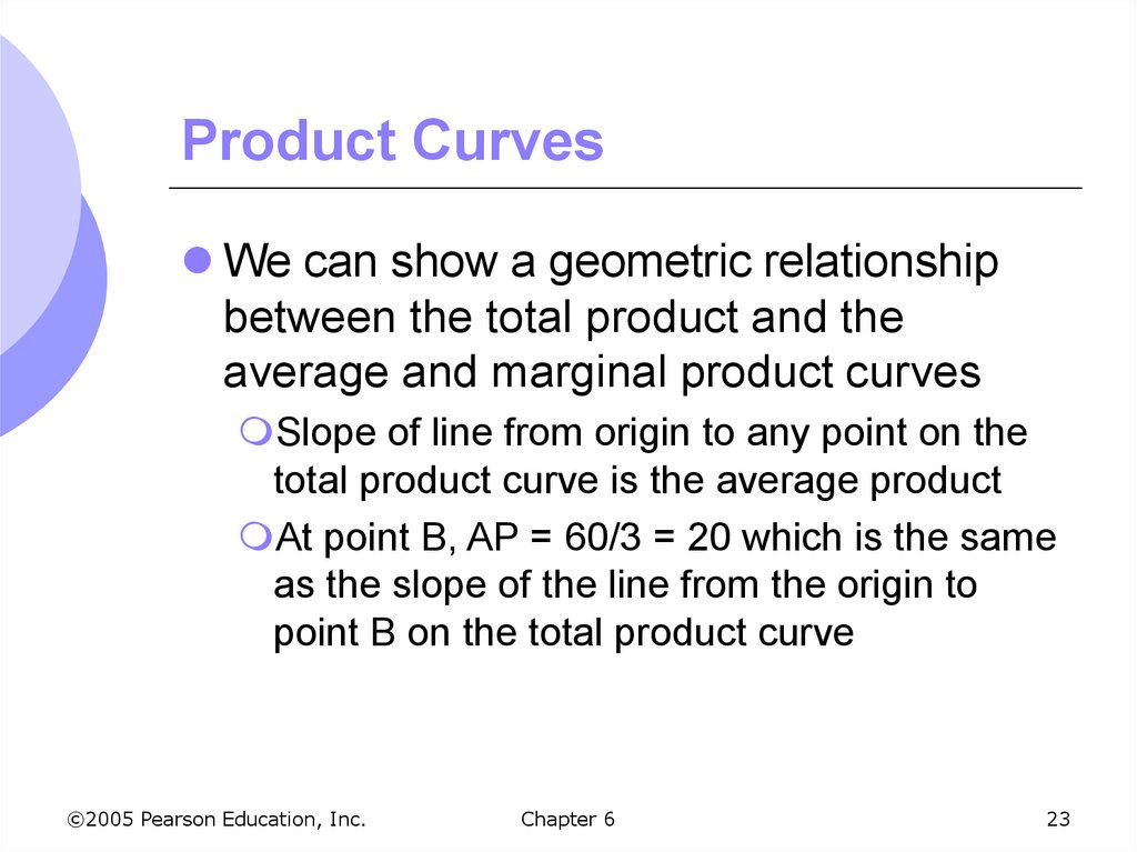
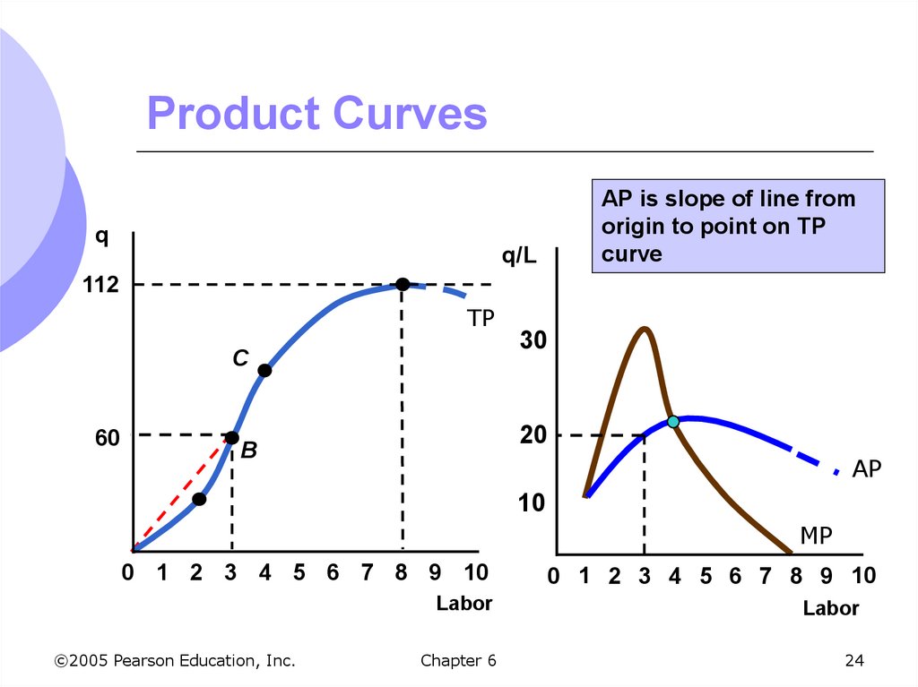
We can show a geometric relationship
between the total product and the
average and marginal product curves
Slope of line from origin to any point on the
total product curve is the average product
At point B, AP = 60/3 = 20 which is the same
as the slope of the line from the origin to
point B on the total product curve
©2005 Pearson Education, Inc.
Chapter 6
23

24. Product Curves

q
AP is slope of line from
origin to point on TP
curve
q/L
112
TP
C
60
30
20
B
AP
10
MP
0 1 2 3 4 5 6 7 8 9 10
©2005 Pearson Education, Inc.
0 1 2 3 4 5 6 7 8 9 10
Labor
Labor
Chapter 6
24

25. Product Curves

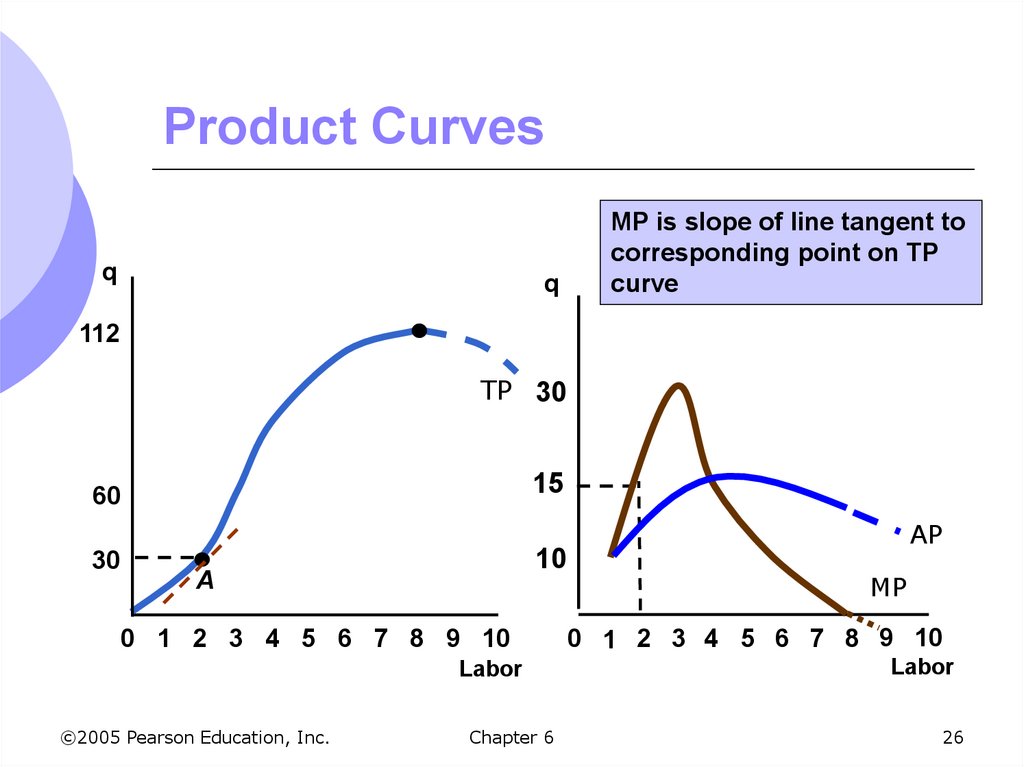
Geometric relationship between total
product and marginal product
The marginal product is the slope of the line
tangent to any corresponding point on the
total product curve
For 2 units of labor, MP = 30/2 = 15 which is
slope of total product curve at point A
©2005 Pearson Education, Inc.
Chapter 6
25

26. Product Curves

q
q
MP is slope of line tangent to
corresponding point on TP
curve
112
TP 30
15
60
30
10
A
AP
MP
0 1 2 3 4 5 6 7 8 9 10
0 1 2 3 4 5 6 7 8 9 10
Labor
Labor
©2005 Pearson Education, Inc.
Chapter 6
26

27. Production: One Variable Input

From the previous example, we can see
that as we increase labor the additional
output produced declines
Law of Diminishing Marginal Returns:
As the use of an input increases with
other inputs fixed, the resulting additions
to output will eventually decrease
©2005 Pearson Education, Inc.
Chapter 6
27

28. Law of Diminishing Marginal Returns

When the use of labor input is small and
capital is fixed, output increases
considerably since workers can begin to
specialize and MP of labor increases
When the use of labor input is large,
some workers become less efficient and
MP of labor decreases
©2005 Pearson Education, Inc.
Chapter 6
28

29. Law of Diminishing Marginal Returns

Typically applies only for the short run
when one variable input is fixed
Can be used for long-run decisions to
evaluate the trade-offs of different plant
configurations
Assumes the quality of the variable input
is constant
©2005 Pearson Education, Inc.
Chapter 6
29

30. Law of Diminishing Marginal Returns

Easily confused with negative returns –
decreases in output
Explains a declining marginal product,
not necessarily a negative one
Additional output can be declining while total
output is increasing
©2005 Pearson Education, Inc.
Chapter 6
30

31. Law of Diminishing Marginal Returns

Assumes a constant technology
Changes in technology will cause shifts in
the total product curve
More output can be produced with same
inputs
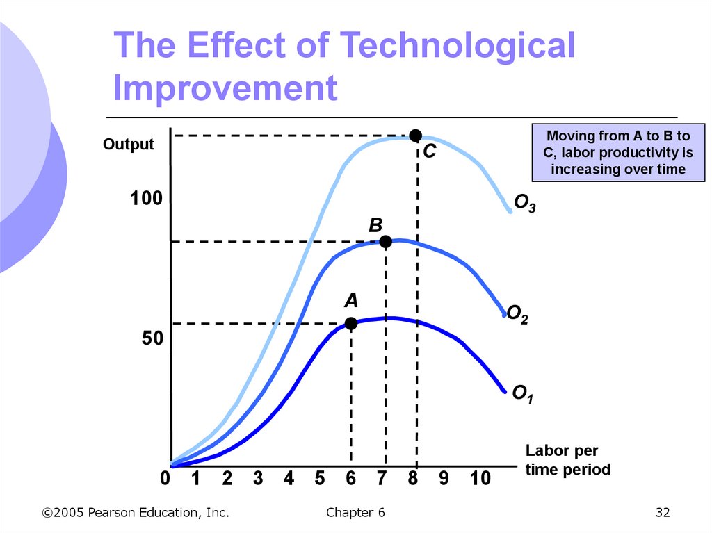
Labor productivity can increase if there are
improvements in technology, even though
any given production process exhibits
diminishing returns to labor
©2005 Pearson Education, Inc.
Chapter 6
31

32. The Effect of Technological Improvement

Output
Moving from A to B to
C, labor productivity is
increasing over time
C
100
O3
B
A
O2
50
O1
0 1
2 3
©2005 Pearson Education, Inc.
4
5 6
7 8
Chapter 6
9
10
Labor per
time period
32

33. Malthus and the Food Crisis

Malthus predicted mass hunger and
starvation as diminishing returns limited
agricultural output and the population
continued to grow
Why did Malthus’ prediction fail?
Did not take into account changes in
technology
Although he was right about diminishing
marginal returns to labor
©2005 Pearson Education, Inc.
Chapter 6
33

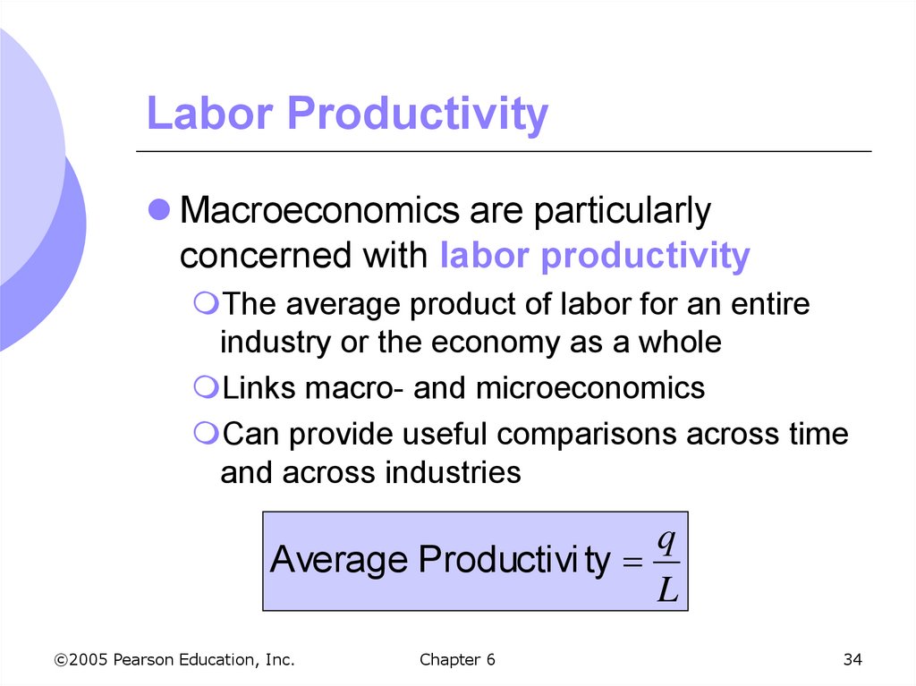
34. Labor Productivity

Macroeconomics are particularly
concerned with labor productivity
The average product of labor for an entire
industry or the economy as a whole
Links macro- and microeconomics
Can provide useful comparisons across time
and across industries
q
Average Productivi ty
L
©2005 Pearson Education, Inc.
Chapter 6
34

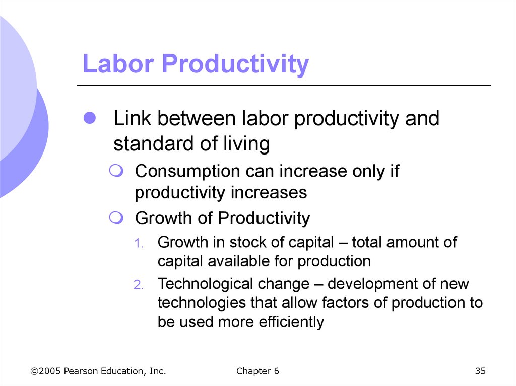
35. Labor Productivity

Link between labor productivity and
standard of living
Consumption can increase only if
productivity increases
Growth of Productivity
Growth in stock of capital – total amount of
capital available for production
2. Technological change – development of new
technologies that allow factors of production to
be used more efficiently
1.
©2005 Pearson Education, Inc.
Chapter 6
35

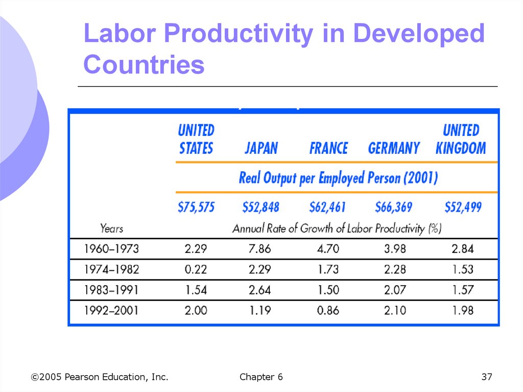
36. Labor Productivity

Trends in Productivity
Labor productivity and productivity growth
have differed considerably across countries
U.S. productivity is growing at a slower rate
than other countries
Productivity growth in developed countries
has been decreasing
Given the central role of productivity in
standards of living, understanding
differences across countries is important
©2005 Pearson Education, Inc.
Chapter 6
36

37. Labor Productivity in Developed Countries

©2005 Pearson Education, Inc.
Chapter 6
37

38. Productivity Growth in US

Why has productivity growth slowed
down?
1. Growth in the stock of capital is the primary
determinant of the growth in productivity
2. Rate of capital accumulation (US) was
slower than other developed countries
because they had to rebuild after WWII
3. Depletion of natural resources
4. Environmental regulations
©2005 Pearson Education, Inc.
Chapter 6
38

39. Production: Two Variable Inputs

Firm can produce output by combining
different amounts of labor and capital
In the long run, capital and labor are both
variable
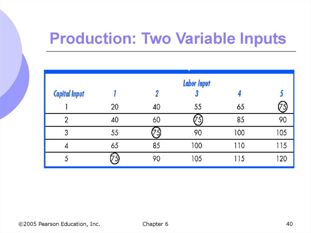
We can look at the output we can
achieve with different combinations of
capital and labor – Table 6.4
©2005 Pearson Education, Inc.
Chapter 6
39

40. Production: Two Variable Inputs

©2005 Pearson Education, Inc.
Chapter 6
40

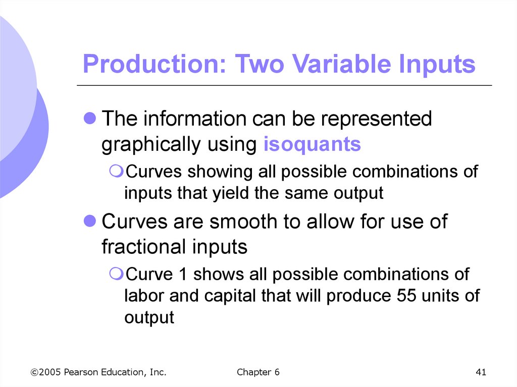
41. Production: Two Variable Inputs

The information can be represented
graphically using isoquants
Curves showing all possible combinations of
inputs that yield the same output
Curves are smooth to allow for use of
fractional inputs
Curve 1 shows all possible combinations of
labor and capital that will produce 55 units of
output
©2005 Pearson Education, Inc.
Chapter 6
41

42. Isoquant Map

E
Capital 5
per year
Ex: 55 units of output
can be produced with
3K & 1L (pt. A)
OR
1K & 3L (pt. D)
4
3
A
B
C
2
q3 = 90
D
1
q2 = 75
q1 = 55
1
©2005 Pearson Education, Inc.
2
3
Chapter 6
4
5
Labor per year
42

43. Production: Two Variable Inputs

Diminishing Returns to Labor with
Isoquants
Holding capital at 3 and increasing labor
from 0 to 1 to 2 to 3
Output increases at a decreasing rate (0, 55,
20, 15) illustrating diminishing marginal
returns from labor in the short run and long
run
©2005 Pearson Education, Inc.
Chapter 6
43

44. Production: Two Variable Inputs

Diminishing Returns to Capital with
Isoquants
Holding labor constant at 3 increasing
capital from 0 to 1 to 2 to 3
Output increases at a decreasing rate (0, 55,
20, 15) due to diminishing returns from
capital in short run and long run
©2005 Pearson Education, Inc.
Chapter 6
44

45. Diminishing Returns

Capital 5
per year
Increasing labor
holding capital
constant (A, B, C)
OR
Increasing capital
holding labor constant
(E, D, C
4
3
A
B
C
D
2
q3 = 90
E
1
q2 = 75
q1 = 55
1
©2005 Pearson Education, Inc.
2
3
Chapter 6
4
5
Labor per year
45

46. Production: Two Variable Inputs

Substituting Among Inputs
Companies must decide what combination of
inputs to use to produce a certain quantity of
output
There is a trade-off between inputs, allowing
them to use more of one input and less of
another for the same level of output
©2005 Pearson Education, Inc.
Chapter 6
46

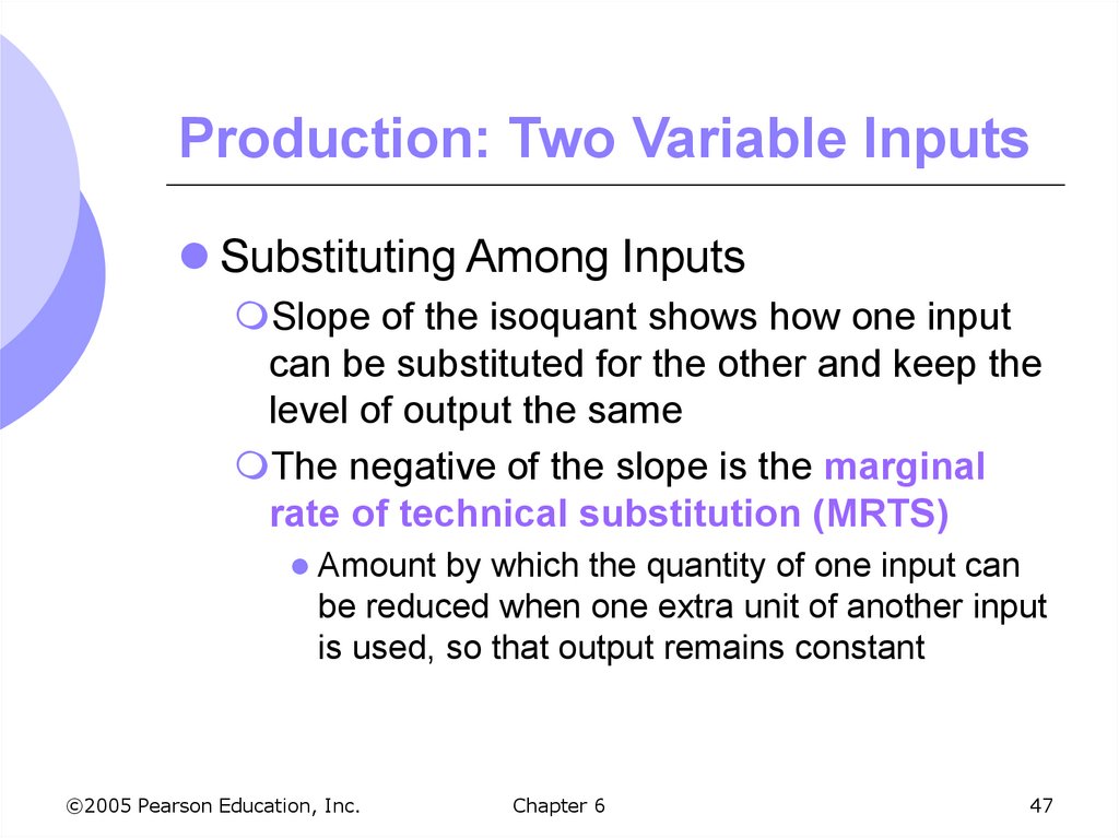
47. Production: Two Variable Inputs

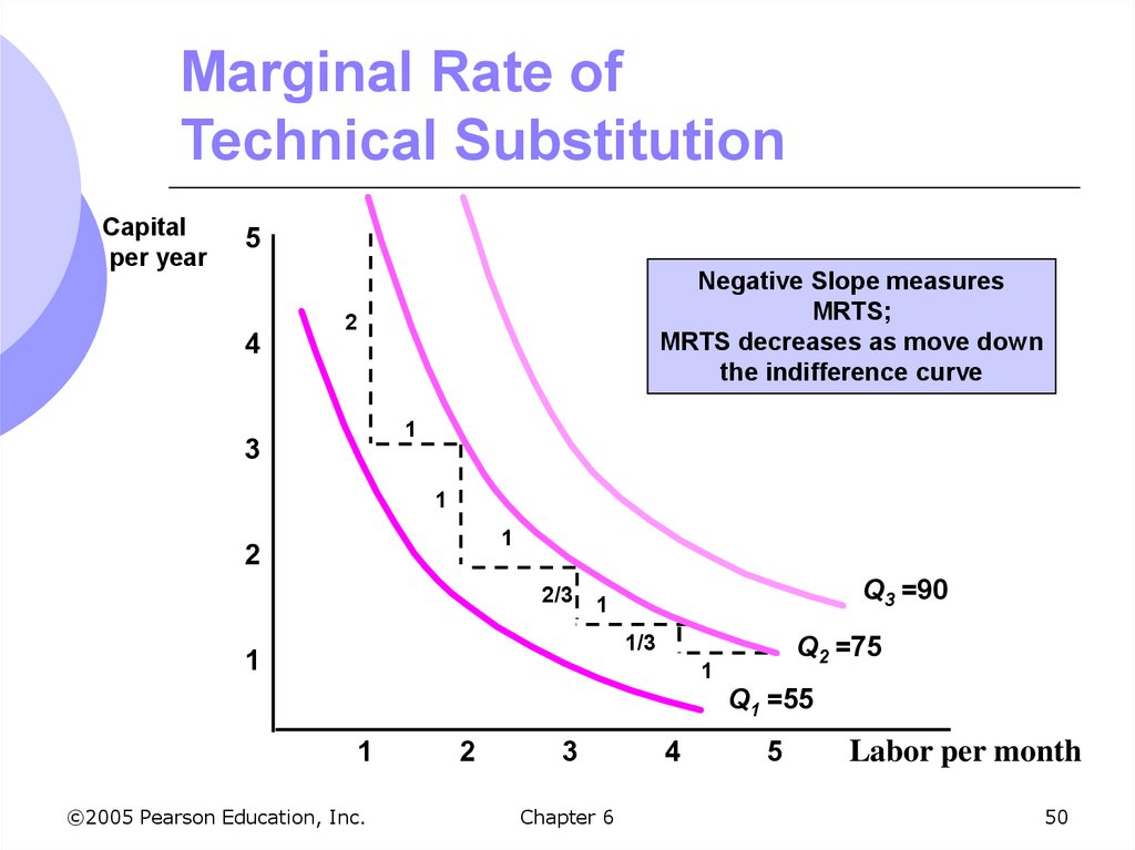
Substituting Among Inputs
Slope of the isoquant shows how one input
can be substituted for the other and keep the
level of output the same
The negative of the slope is the marginal
rate of technical substitution (MRTS)
Amount by which the quantity of one input can
be reduced when one extra unit of another input
is used, so that output remains constant
©2005 Pearson Education, Inc.
Chapter 6
47

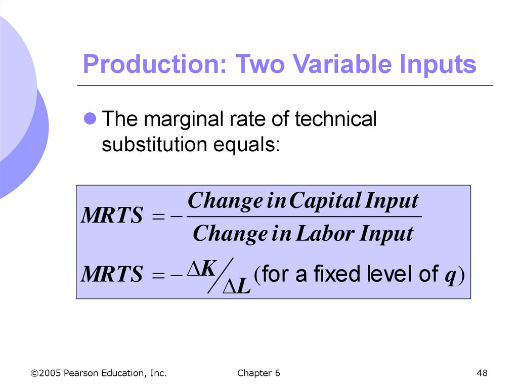
48. Production: Two Variable Inputs

The marginal rate of technical
substitution equals:
Change in Capital Input
MRTS
Change in Labor Input
MRTS K
(for a fixed level of q )
L
©2005 Pearson Education, Inc.
Chapter 6
48

49. Production: Two Variable Inputs

As labor increases to replace capital
Labor becomes relatively less productive
Capital becomes relatively more productive
Need less capital to keep output constant
Isoquant becomes flatter
©2005 Pearson Education, Inc.
Chapter 6
49

50. Marginal Rate of Technical Substitution

Capital
per year
5
4
Negative Slope measures
MRTS;
MRTS decreases as move down
the indifference curve
2
1
3
1
1
2
2/3
Q3 =90
1
1/3
1
Q2 =75
1
Q1 =55
1
©2005 Pearson Education, Inc.
2
3
Chapter 6
4
5
Labor per month
50

51. MRTS and Isoquants

We assume there is diminishing MRTS
Increasing labor in one unit increments from 1 to 5
results in a decreasing MRTS from 1 to 1/2
Productivity of any one input is limited
Diminishing MRTS occurs because of
diminishing returns and implies isoquants are
convex
There is a relationship between MRTS and
marginal products of inputs
©2005 Pearson Education, Inc.
Chapter 6
51

52. MRTS and Marginal Products

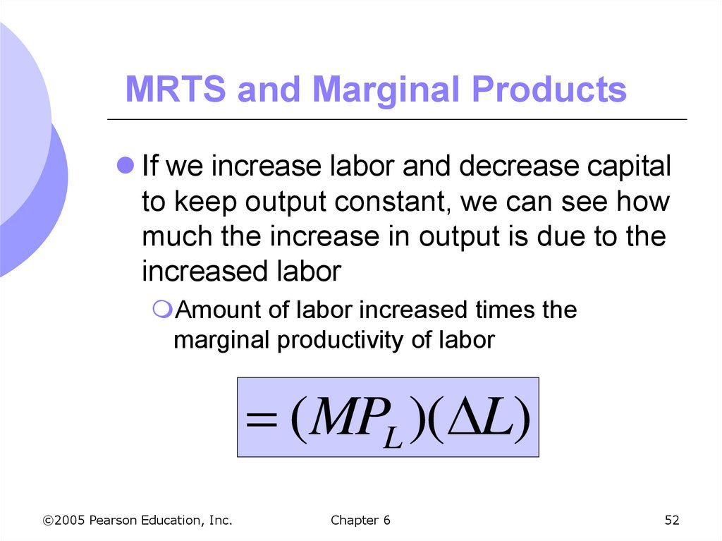
If we increase labor and decrease capital
to keep output constant, we can see how
much the increase in output is due to the
increased labor
Amount of labor increased times the
marginal productivity of labor
(MPL )( L)
©2005 Pearson Education, Inc.
Chapter 6
52

53. MRTS and Marginal Products

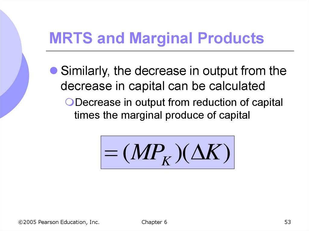
Similarly, the decrease in output from the
decrease in capital can be calculated
Decrease in output from reduction of capital
times the marginal produce of capital
(MPK )( K )
©2005 Pearson Education, Inc.
Chapter 6
53

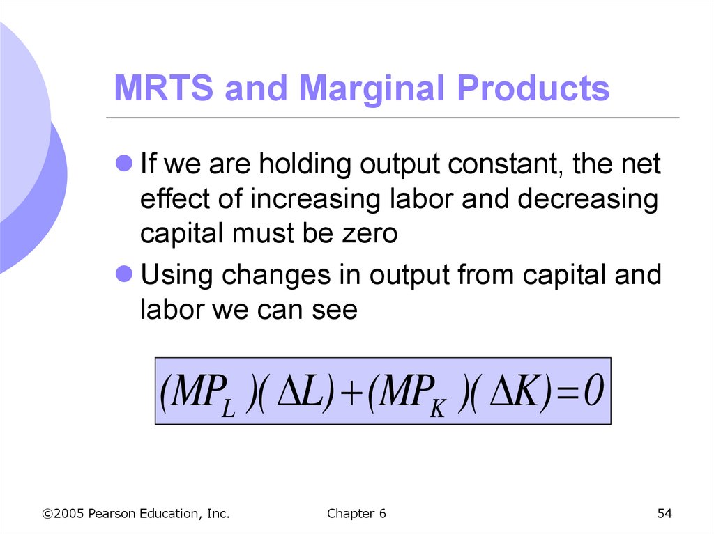
54. MRTS and Marginal Products

If we are holding output constant, the net
effect of increasing labor and decreasing
capital must be zero
Using changes in output from capital and
labor we can see
(MPL )( L) (MPK )( K) 0
©2005 Pearson Education, Inc.
Chapter 6
54

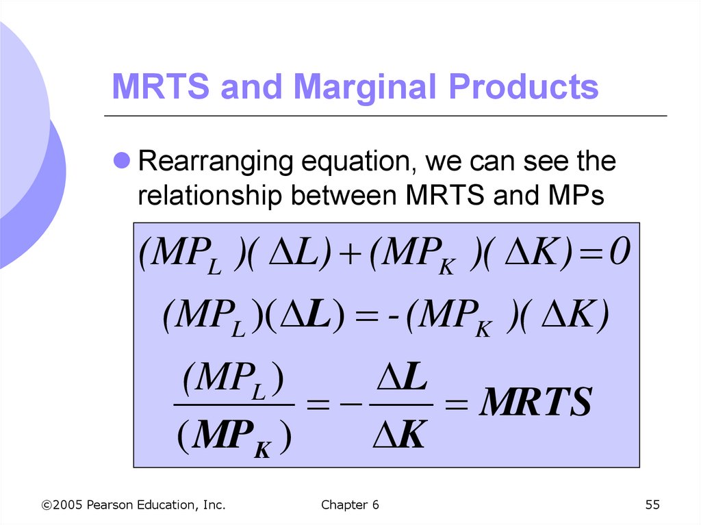
55. MRTS and Marginal Products

Rearranging equation, we can see the
relationship between MRTS and MPs
(MPL )( L) (MPK )( K) 0
(MPL )( L) - (MPK )( K)
(MPL )
L
MRTS
( MPK )
K
©2005 Pearson Education, Inc.
Chapter 6
55

56. Isoquants: Special Cases

Two extreme cases show the possible
range of input substitution in production
1. Perfect substitutes
MRTS is constant at all points on isoquant
Same output can be produced with a lot of
capital or a lot of labor or a balanced mix
©2005 Pearson Education, Inc.
Chapter 6
56

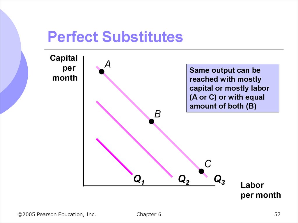
57. Perfect Substitutes

Capital
per
month
A
Same output can be
reached with mostly
capital or mostly labor
(A or C) or with equal
amount of both (B)
B
C
Q1
©2005 Pearson Education, Inc.
Chapter 6
Q2
Q3
Labor
per month
57

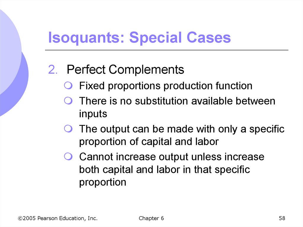
58. Isoquants: Special Cases

2. Perfect Complements
Fixed proportions production function
There is no substitution available between
inputs
The output can be made with only a specific
proportion of capital and labor
Cannot increase output unless increase
both capital and labor in that specific
proportion
©2005 Pearson Education, Inc.
Chapter 6
58

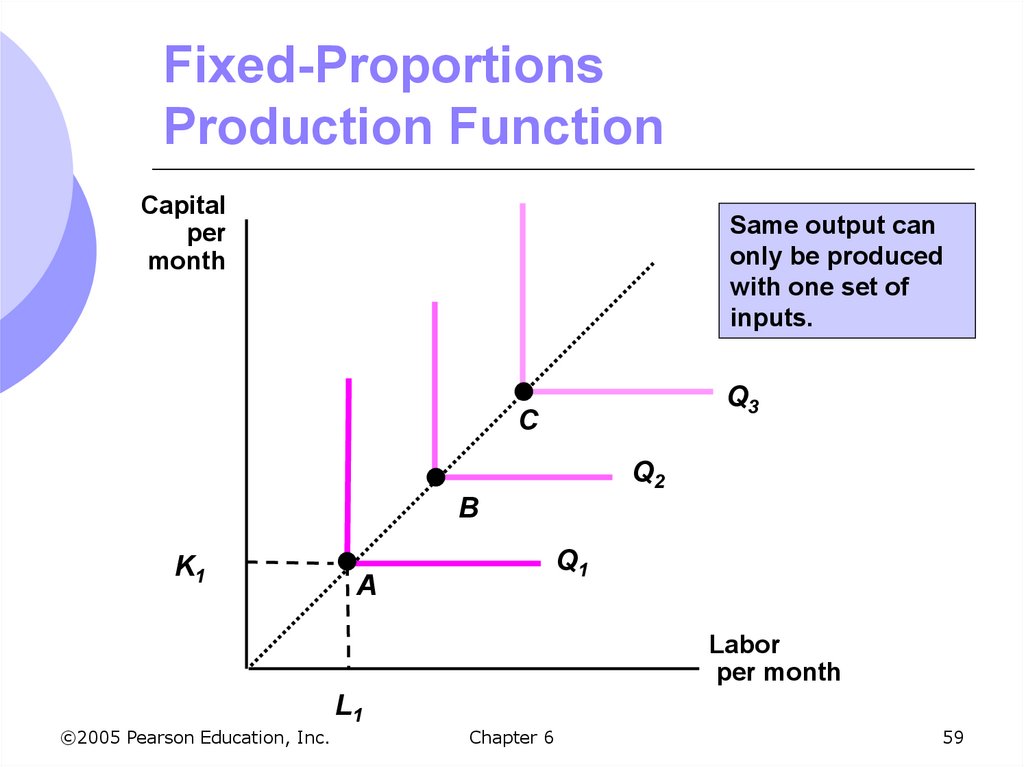
59. Fixed-Proportions Production Function

Capital
per
month
Same output can
only be produced
with one set of
inputs.
Q3
C
Q2
B
K1
Q1
A
Labor
per month
L1
©2005 Pearson Education, Inc.
Chapter 6
59

60. A Production Function for Wheat

Farmers can produce crops with different
combinations of capital and labor
Crops in US are typically grown with capitalintensive technology
Crops in developing countries grown with
labor-intensive productions
Can show the different options of crop
production with isoquants
©2005 Pearson Education, Inc.
Chapter 6
60

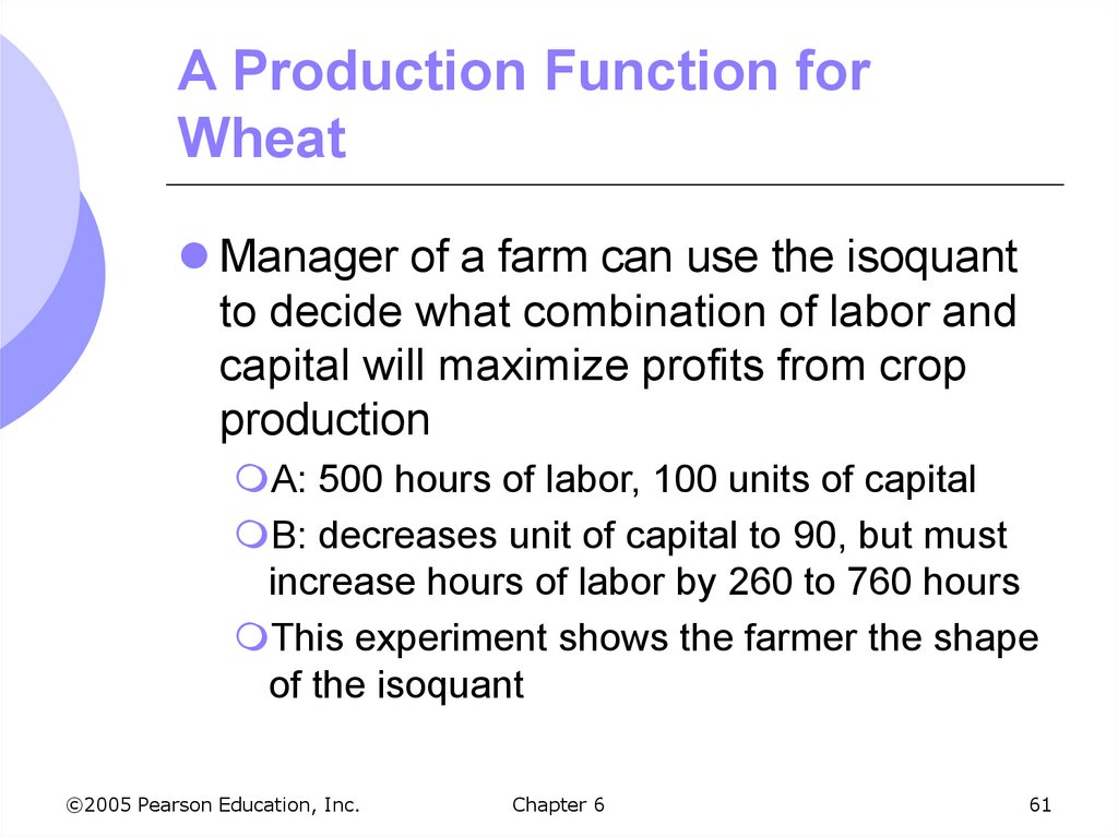
61. A Production Function for Wheat

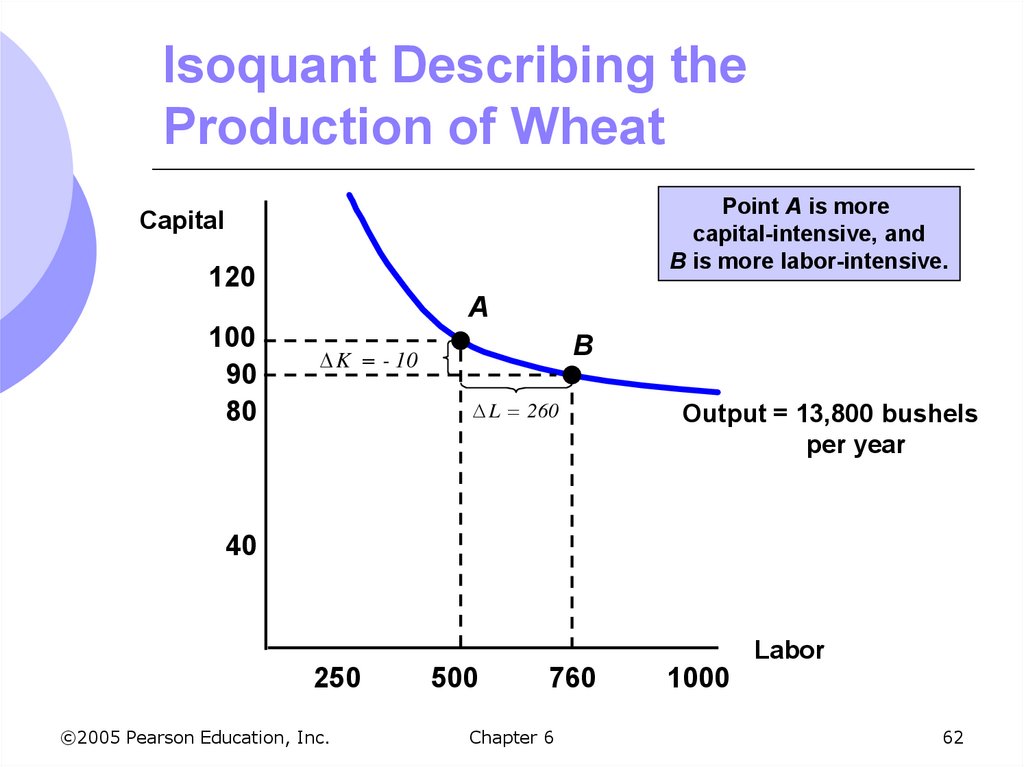
Manager of a farm can use the isoquant
to decide what combination of labor and
capital will maximize profits from crop
production
A: 500 hours of labor, 100 units of capital
B: decreases unit of capital to 90, but must
increase hours of labor by 260 to 760 hours
This experiment shows the farmer the shape
of the isoquant
©2005 Pearson Education, Inc.
Chapter 6
61

62. Isoquant Describing the Production of Wheat

Point A is more
capital-intensive, and
B is more labor-intensive.
Capital
120
A
100
90
80
B
K - 10
L 260
Output = 13,800 bushels
per year
40
Labor
250
©2005 Pearson Education, Inc.
500
760
Chapter 6
1000
62

63. A Production Function for Wheat

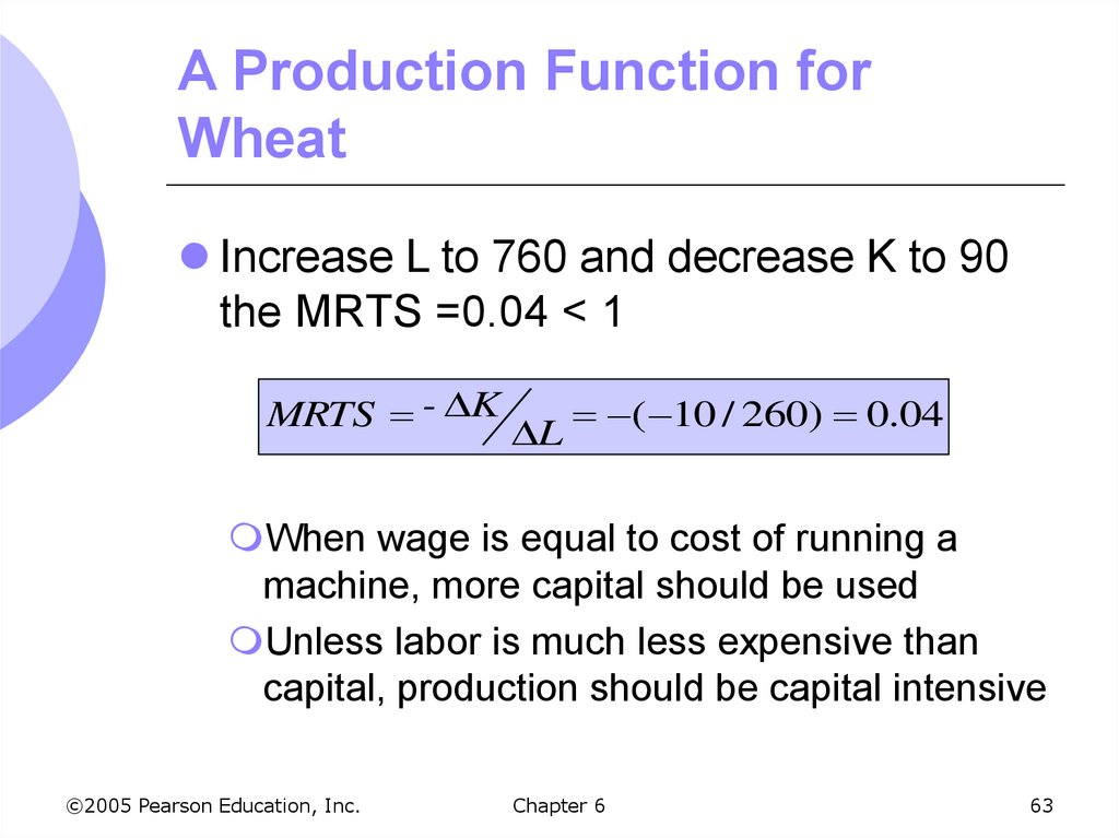
Increase L to 760 and decrease K to 90
the MRTS =0.04 < 1
MRTS - K
L
( 10 / 260) 0.04
When wage is equal to cost of running a
machine, more capital should be used
Unless labor is much less expensive than
capital, production should be capital intensive
©2005 Pearson Education, Inc.
Chapter 6
63

64. Returns to Scale

In addition to discussing the tradeoff
between inputs to keep production the
same
How does a firm decide, in the long run,
the best way to increase output?
Can change the scale of production by
increasing all inputs in proportion
If double inputs, output will most likely
increase but by how much?
©2005 Pearson Education, Inc.
Chapter 6
64

65. Returns to Scale

Rate at which output increases as inputs
are increased proportionately
Increasing returns to scale
Constant returns to scale
Decreasing returns to scale
©2005 Pearson Education, Inc.
Chapter 6
65

66. Returns to Scale

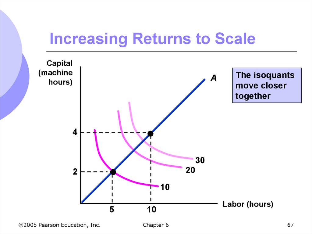
Increasing returns to scale: output
more than doubles when all inputs are
doubled
Larger output associated with lower cost
(cars)
One firm is more efficient than many (utilities)
The isoquants get closer together
©2005 Pearson Education, Inc.
Chapter 6
66

67. Increasing Returns to Scale

Capital
(machine
hours)
A
The isoquants
move closer
together
4
30
20
2
10
5
©2005 Pearson Education, Inc.
10
Chapter 6
Labor (hours)
67

68. Returns to Scale

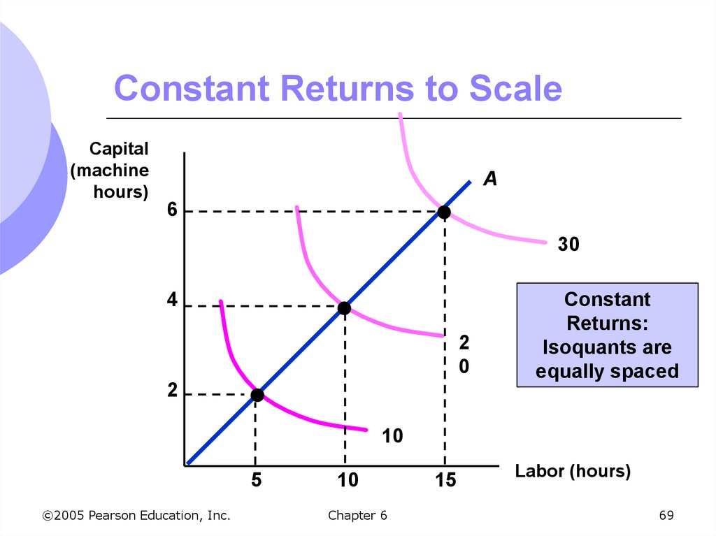
Constant returns to scale: output
doubles when all inputs are doubled
Size does not affect productivity
May have a large number of producers
Isoquants are equidistant apart
©2005 Pearson Education, Inc.
Chapter 6
68

69. Constant Returns to Scale

Capital
(machine
hours)
A
6
30
4
2
0
2
Constant
Returns:
Isoquants are
equally spaced
10
5
©2005 Pearson Education, Inc.
10
Chapter 6
15
Labor (hours)
69

70. Returns to Scale

Decreasing returns to scale: output
less than doubles when all inputs are
doubled
Decreasing efficiency with large size
Reduction of entrepreneurial abilities
Isoquants become farther apart
©2005 Pearson Education, Inc.
Chapter 6
70

71. Decreasing Returns to Scale

Capital
(machine
hours)
A
4
20
2
Decreasing Returns:
Isoquants get further
apart
10
5
©2005 Pearson Education, Inc.
10
Chapter 6
Labor (hours)
71

72. Returns to Scale: Carpet Industry

The carpet industry has grown from a small
industry to a large industry with some very large
firms
There are four relatively large manufacturers
along with a number of smaller ones
Growth has come from
Increased consumer demand
More efficient production reducing costs
Innovation and competition have reduced real prices
©2005 Pearson Education, Inc.
Chapter 6
72

73. The U.S. Carpet Industry

©2005 Pearson Education, Inc.
Chapter 6
73

74. Returns to Scale: Carpet Industry

Some growth can be explained by
returns to scale
Carpet production is highly capital
intensive
Heavy upfront investment in machines for
carpet production
Increases in scale of operating have
occurred by putting in larger and more
efficient machines into larger plants
©2005 Pearson Education, Inc.
Chapter 6
74

75. Returns to Scale: Carpet Industry Results

1. Large Manufacturers
Increases in machinery and labor
Doubling inputs has more than doubled
output
Economies of scale exist for large
producers
©2005 Pearson Education, Inc.
Chapter 6
75

76. Returns to Scale: Carpet Industry Results

2. Small Manufacturers
Small increases in scale have little or no
impact on output
Proportional increases in inputs increase
output proportionally
Constant returns to scale for small
producers
©2005 Pearson Education, Inc.
Chapter 6
76

77. Returns to Scale: Carpet Industry

From this we can see that the carpet
industry is one where:
1. There are constant returns to scale for
relatively small plants
2. There are increasing returns to scale for
relatively larger plants
These are limited, however
Eventually reach decreasing returns
©2005 Pearson Education, Inc.
Chapter 6
77