

 marketing
Similar presentations:


")


Business Analytics
1.
Chapter 2Describing the Distribution of a Single Variable
© 2017 Cengage Learning. All Rights Reserved. May not be scanned, copied or duplicated, or posted to a publicly accessible website, in whole or in part.
2.
Описание распределения одной переменнойОписание распределения одной переменной
© 2017 Cengage Learning. All Rights Reserved. May not be scanned, copied or duplicated, or posted to a publicly accessible website, in whole or in part.
3.
2-1 ВведениеНаша цель - представить данные в понятной для
людей форме. Для этого используются следующие
инструменты:
Графики: гистограммы, круговые диаграммы,
гистограммы, точечные диаграммы и графики временных
рядов.
Сводные числовые показатели: количество, процентное
соотношение, средние значения и меры изменчивости.
Таблицы итоговых показателей: итоговые, средние,
количественные и сгруппированные по категориям
Сложно обобщить(довести) данные (описать важную
информацию).
© 2017 Cengage Learning. All Rights Reserved. May not be scanned, copied or duplicated, or posted to a publicly accessible website, in whole or in part.
4.
2-1 IntroductionOur goal is to present data in a form that makes
sense to people. Tools that are used to do this include:
Graphs: bar charts, pie charts, histograms, scatter
charts, and time series graphs
Numerical summary measures: counts, percentages,
averages, and measures of variability
Tables of summary measures: totals, averages, counts,
and grouped by categories
It is a challenge to summarize the data (Describing
important information)
© 2017 Cengage Learning. All Rights Reserved. May not be scanned, copied or duplicated, or posted to a publicly accessible website, in whole or in part.
5.
2-2 Основные концепцииНесколько важных концепций
Популяции и образцы
Наборы данных
Переменные и наблюдения
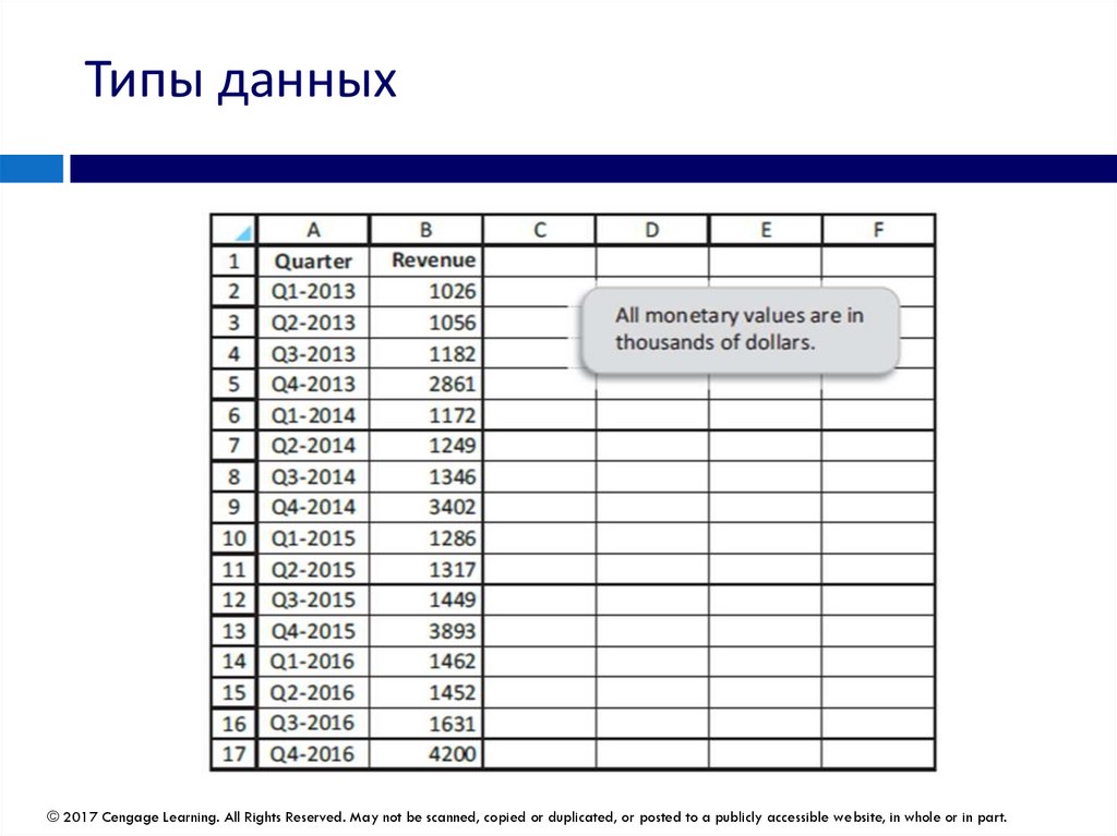
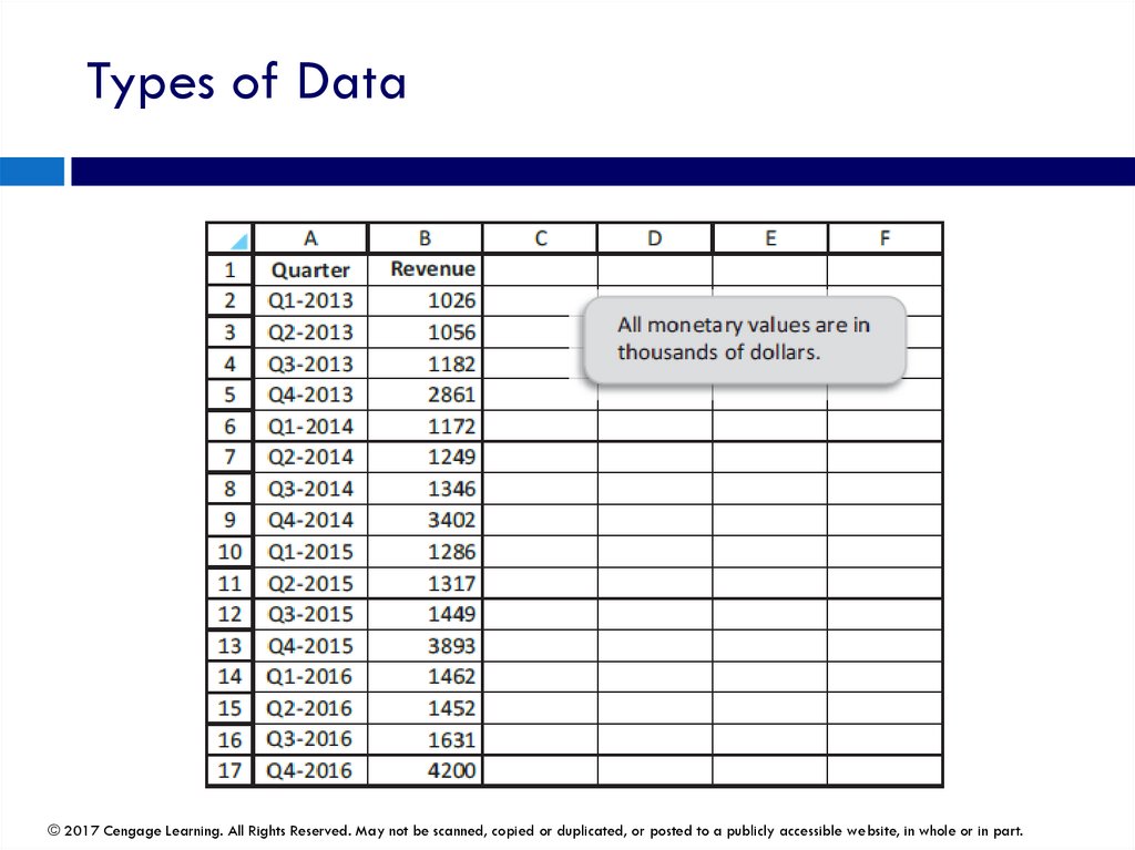
Типы данных
© 2017 Cengage Learning. All Rights Reserved. May not be scanned, copied or duplicated, or posted to a publicly accessible website, in whole or in part.
6.
2-2 Basic ConceptsSeveral important concepts
Populations and samples
Data sets
Variables and observations
Types of data
© 2017 Cengage Learning. All Rights Reserved. May not be scanned, copied or duplicated, or posted to a publicly accessible website, in whole or in part.
7.
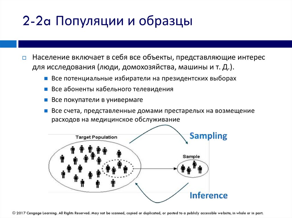
2-2a Популяции и образцыНаселение включает в себя все объекты, представляющие интерес
для исследования (люди, домохозяйства, машины и т. Д.).
Все потенциальные избиратели на президентских выборах
Все абоненты кабельного телевидения
Все покупатели в универмаге
Все счета, представленные домами престарелых на возмещение
расходов на медицинское обслуживание
© 2017 Cengage Learning. All Rights Reserved. May not be scanned, copied or duplicated, or posted to a publicly accessible website, in whole or in part.
8.
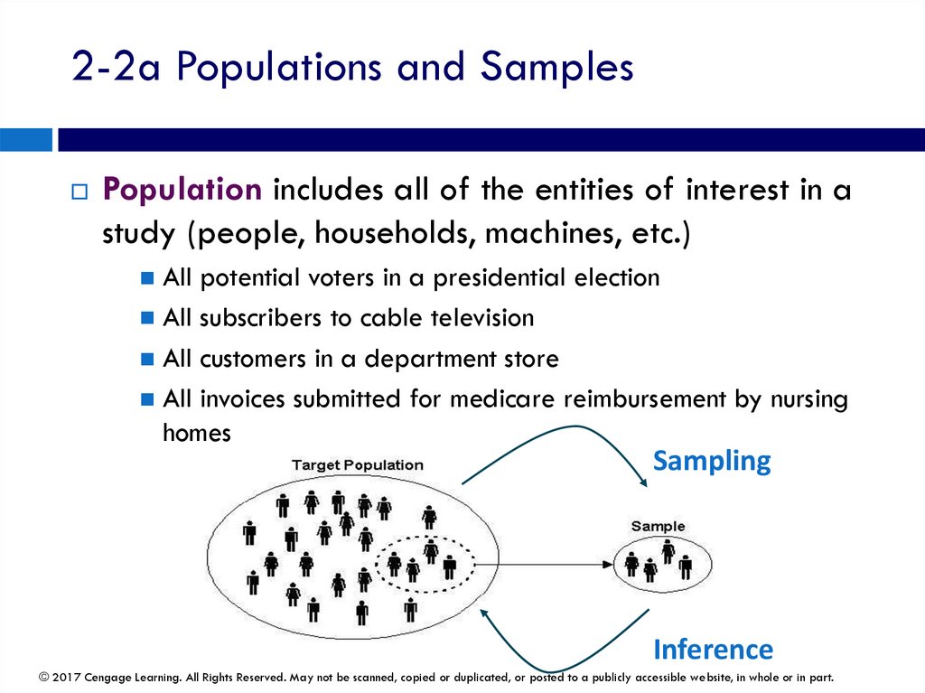
2-2a Populations and SamplesPopulation includes all of the entities of interest in a
study (people, households, machines, etc.)
All potential voters in a presidential election
All subscribers to cable television
All customers in a department store
All invoices submitted for medicare reimbursement by nursing
homes
Sampling
Inference
© 2017 Cengage Learning. All Rights Reserved. May not be scanned, copied or duplicated, or posted to a publicly accessible website, in whole or in part.
9.
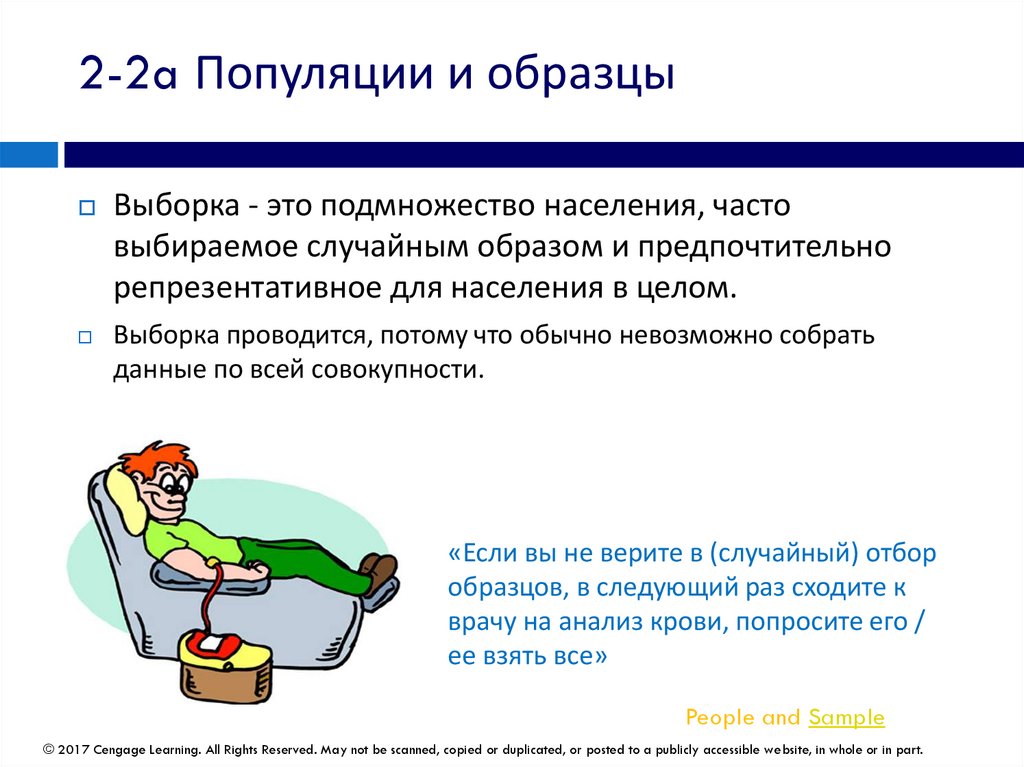
2-2a Популяции и образцыВыборка - это подмножество населения, часто
выбираемое случайным образом и предпочтительно
репрезентативное для населения в целом.
Выборка проводится, потому что обычно невозможно собрать
данные по всей совокупности.
«Если вы не верите в (случайный) отбор
образцов, в следующий раз сходите к
врачу на анализ крови, попросите его /
ее взять все»
People and Sample
© 2017 Cengage Learning. All Rights Reserved. May not be scanned, copied or duplicated, or posted to a publicly accessible website, in whole or in part.
10.
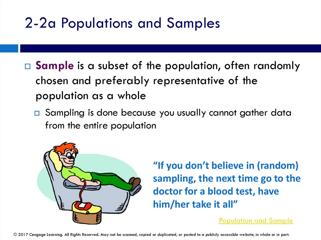
2-2a Populations and SamplesSample is a subset of the population, often randomly
chosen and preferably representative of the
population as a whole
Sampling is done because you usually cannot gather data
from the entire population
“If you don’t believe in (random)
sampling, the next time go to the
doctor for a blood test, have
him/her take it all”
Population and Sample
© 2017 Cengage Learning. All Rights Reserved. May not be scanned, copied or duplicated, or posted to a publicly accessible website, in whole or in part.
11.
2-2a Популяции и образцыПараметр населения - это количество или
статистическая мера всего населения.
Статистика выборки - это любое суммарное
число или статистическая мера выборки.
© 2017 Cengage Learning. All Rights Reserved. May not be scanned, copied or duplicated, or posted to a publicly accessible website, in whole or in part.
12.
2-2a Populations and SamplesPopulation parameter is a quantity or statistical
measure of the entire population
Sample statistic is any summary number or statistical
measure of a sample
© 2017 Cengage Learning. All Rights Reserved. May not be scanned, copied or duplicated, or posted to a publicly accessible website, in whole or in part.
13.
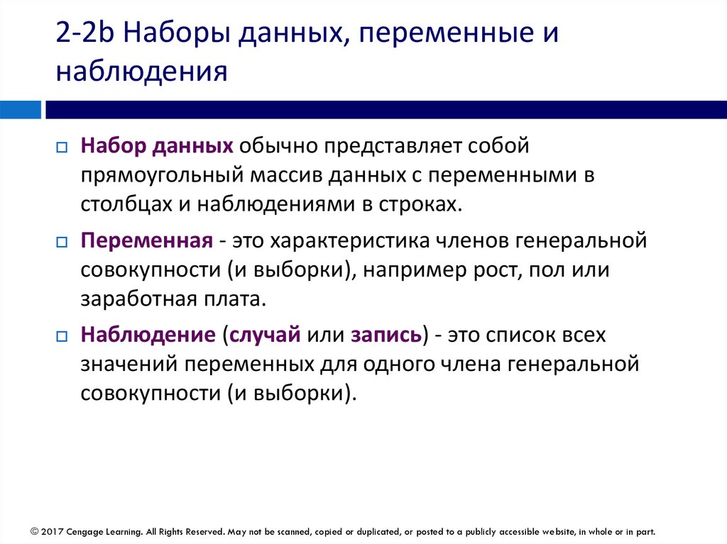
2-2b Наборы данных, переменные инаблюдения
Набор данных обычно представляет собой
прямоугольный массив данных с переменными в
столбцах и наблюдениями в строках.
Переменная - это характеристика членов генеральной
совокупности (и выборки), например рост, пол или
заработная плата.
Наблюдение (случай или запись) - это список всех
значений переменных для одного члена генеральной
совокупности (и выборки).
© 2017 Cengage Learning. All Rights Reserved. May not be scanned, copied or duplicated, or posted to a publicly accessible website, in whole or in part.
14.
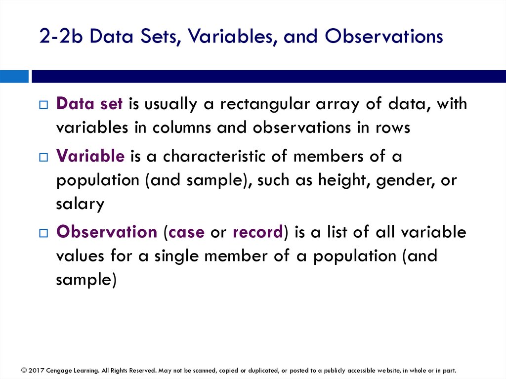
2-2b Data Sets, Variables, and ObservationsData set is usually a rectangular array of data, with
variables in columns and observations in rows
Variable is a characteristic of members of a
population (and sample), such as height, gender, or
salary
Observation (case or record) is a list of all variable
values for a single member of a population (and
sample)
© 2017 Cengage Learning. All Rights Reserved. May not be scanned, copied or duplicated, or posted to a publicly accessible website, in whole or in part.
15.
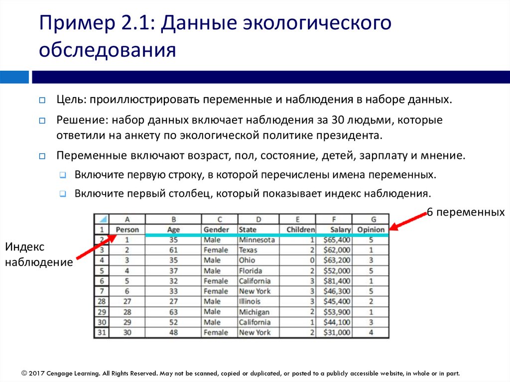
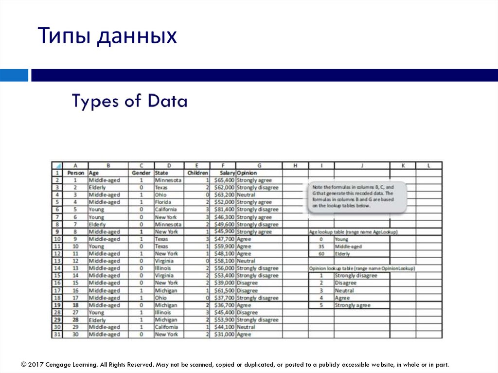
Пример 2.1: Данные экологическогообследования
Цель: проиллюстрировать переменные и наблюдения в наборе данных.
Решение: набор данных включает наблюдения за 30 людьми, которые
ответили на анкету по экологической политике президента.
Переменные включают возраст, пол, состояние, детей, зарплату и мнение.
Включите первую строку, в которой перечислены имена переменных.
Включите первый столбец, который показывает индекс наблюдения.
6 переменных
Индекс
наблюдение
© 2017 Cengage Learning. All Rights Reserved. May not be scanned, copied or duplicated, or posted to a publicly accessible website, in whole or in part.
16.
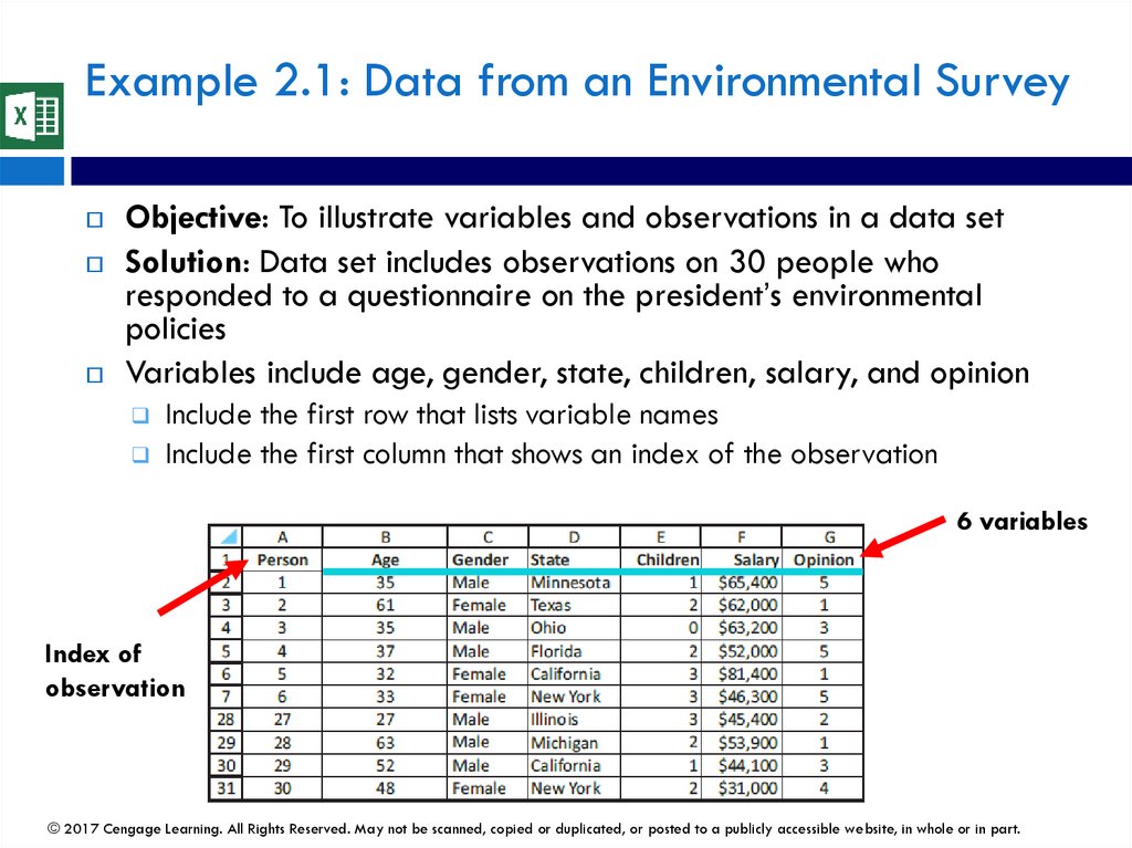
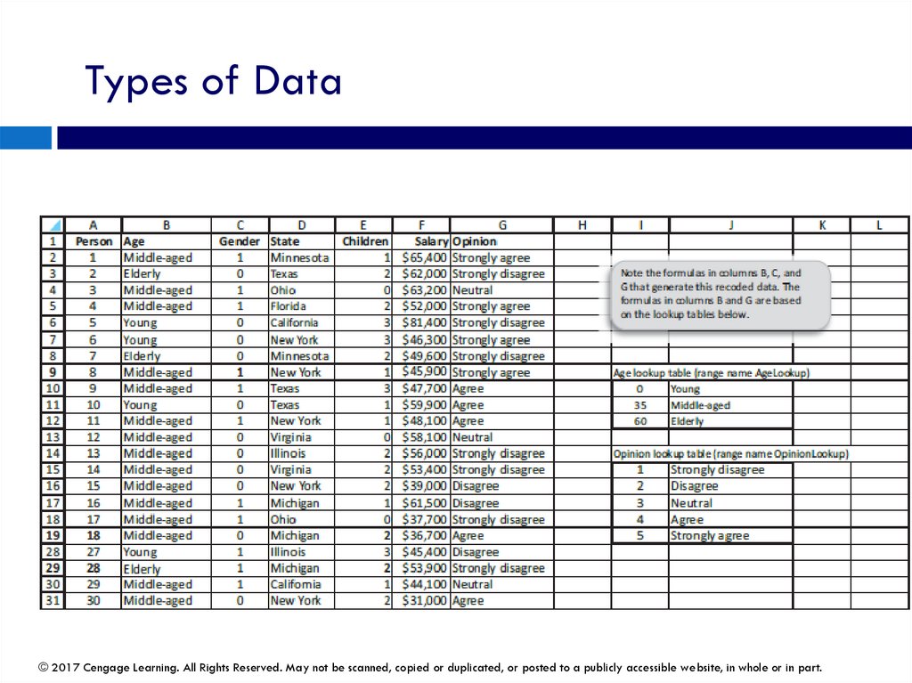
Example 2.1: Data from an Environmental SurveyObjective: To illustrate variables and observations in a data set
Solution: Data set includes observations on 30 people who
responded to a questionnaire on the president’s environmental
policies
Variables include age, gender, state, children, salary, and opinion
Include the first row that lists variable names
Include the first column that shows an index of the observation
6 variables
Index of
observation
© 2017 Cengage Learning. All Rights Reserved. May not be scanned, copied or duplicated, or posted to a publicly accessible website, in whole or in part.
17.
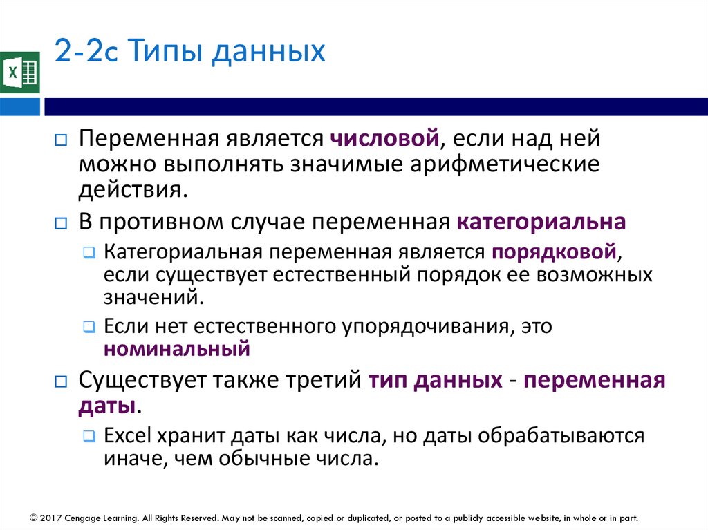
2-2c Типы данныхПеременная является числовой, если над ней
можно выполнять значимые арифметические
действия.
В противном случае переменная категориальна
Категориальная переменная является порядковой,
если существует естественный порядок ее возможных
значений.
Если нет естественного упорядочивания, это
номинальный
Существует также третий тип данных - переменная
даты.
Excel хранит даты как числа, но даты обрабатываются
иначе, чем обычные числа.
© 2017 Cengage Learning. All Rights Reserved. May not be scanned, copied or duplicated, or posted to a publicly accessible website, in whole or in part.
18.
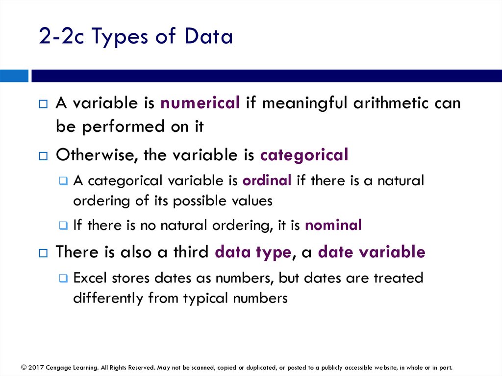
2-2c Types of DataA variable is numerical if meaningful arithmetic can
be performed on it
Otherwise, the variable is categorical
A categorical variable is ordinal if there is a natural
ordering of its possible values
If there is no natural ordering, it is nominal
There is also a third data type, a date variable
Excel stores dates as numbers, but dates are treated
differently from typical numbers
© 2017 Cengage Learning. All Rights Reserved. May not be scanned, copied or duplicated, or posted to a publicly accessible website, in whole or in part.
19.
Четыре шкалы измеренияКатегориальные или качественные переменные
Номинальные:
Порядковые:
© 2017 Cengage Learning. All Rights Reserved. May not be scanned, copied or duplicated, or posted to a publicly accessible website, in whole or in part.
20.
Four Scales of MeasurementCategorical or qualitative variables
Nominal:
Ordinal:
© 2017 Cengage Learning. All Rights Reserved. May not be scanned, copied or duplicated, or posted to a publicly accessible website, in whole or in part.
21.
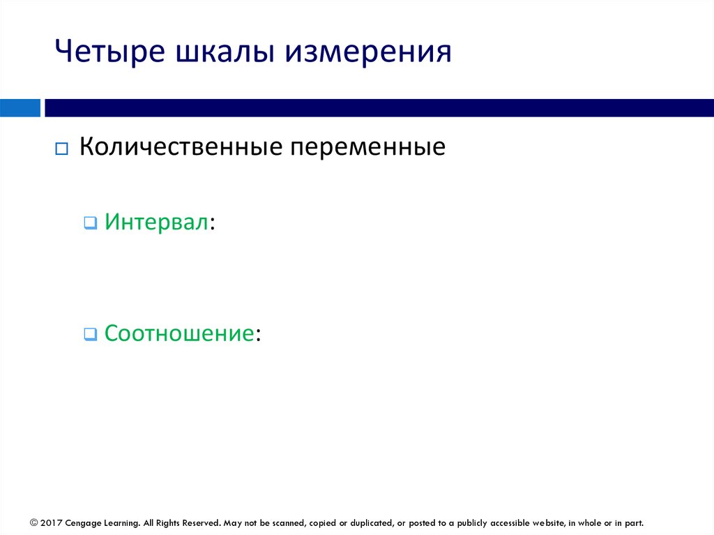
Четыре шкалы измеренияКоличественные переменные
Интервал:
Соотношение:
© 2017 Cengage Learning. All Rights Reserved. May not be scanned, copied or duplicated, or posted to a publicly accessible website, in whole or in part.
22.
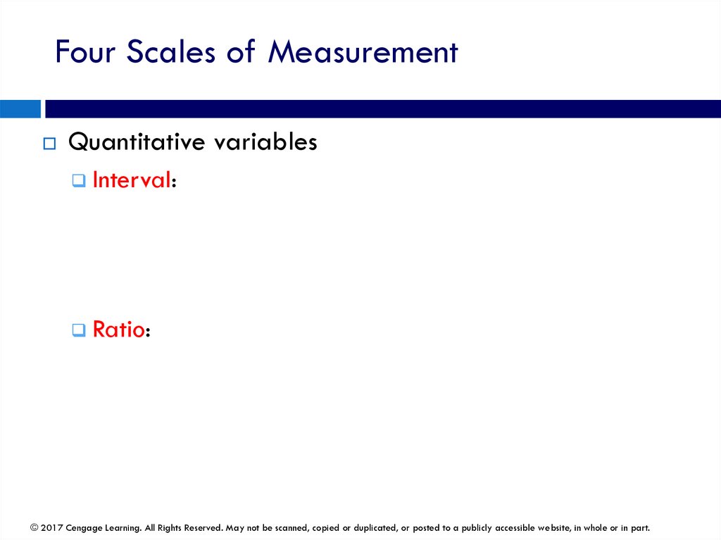
Four Scales of MeasurementQuantitative variables
Interval:
Ratio:
© 2017 Cengage Learning. All Rights Reserved. May not be scanned, copied or duplicated, or posted to a publicly accessible website, in whole or in part.
23.
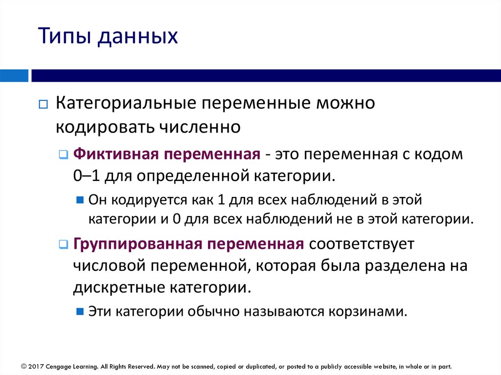
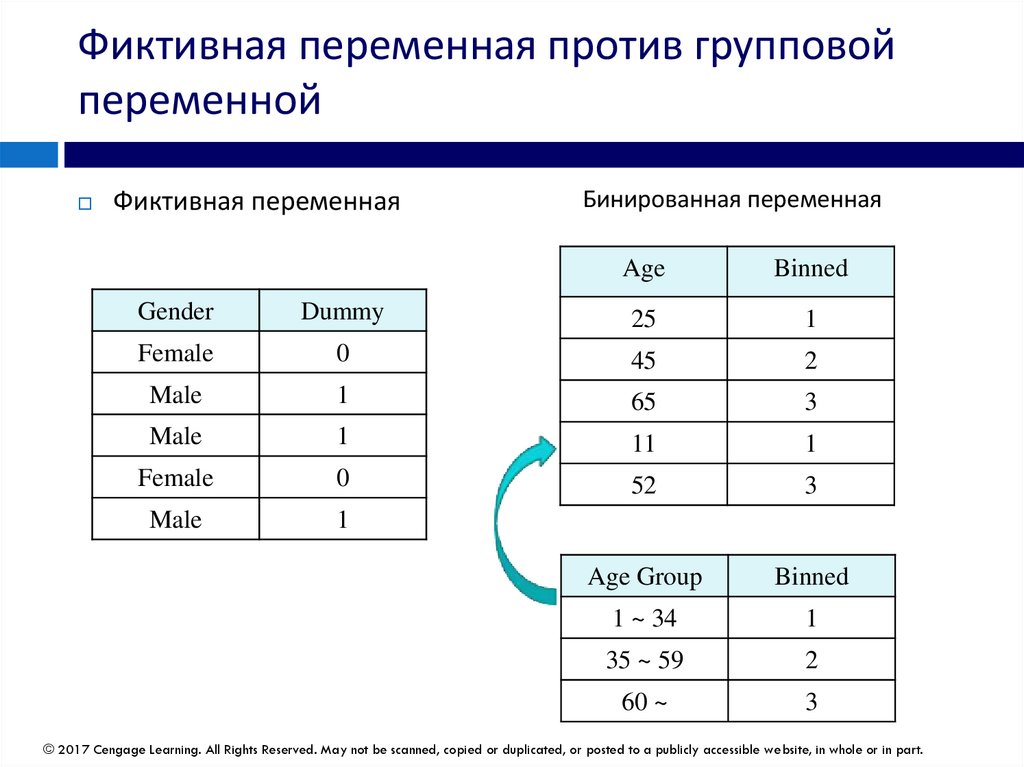
Типы данныхКатегориальные переменные можно
кодировать численно
Фиктивная переменная - это переменная с кодом
0–1 для определенной категории.
Он кодируется как 1 для всех наблюдений в этой
категории и 0 для всех наблюдений не в этой категории.
Группированная переменная соответствует
числовой переменной, которая была разделена на
дискретные категории.
Эти категории обычно называются корзинами.
© 2017 Cengage Learning. All Rights Reserved. May not be scanned, copied or duplicated, or posted to a publicly accessible website, in whole or in part.
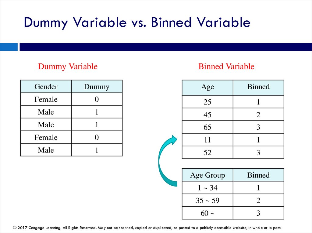
24.
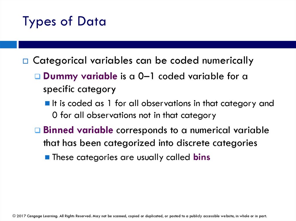
Types of DataCategorical variables can be coded numerically
Dummy variable is a 0–1 coded variable for a
specific category
It is coded as 1 for all observations in that category and
0 for all observations not in that category
Binned variable corresponds to a numerical variable
that has been categorized into discrete categories
These categories are usually called bins
© 2017 Cengage Learning. All Rights Reserved. May not be scanned, copied or duplicated, or posted to a publicly accessible website, in whole or in part.
25.
Фиктивная переменная против групповойпеременной
Фиктивная переменная
Бинированная переменная
Age
Binned
Gender
Dummy
25
1
Female
0
45
2
Male
1
65
3
Male
1
11
1
Female
0
52
3
Male
1
Age Group
Binned
1 ~ 34
1
35 ~ 59
2
60 ~
3
© 2017 Cengage Learning. All Rights Reserved. May not be scanned, copied or duplicated, or posted to a publicly accessible website, in whole or in part.
26.
Dummy Variable vs. Binned VariableDummy Variable
Binned Variable
Gender
Dummy
Age
Binned
Female
0
25
1
Male
1
45
2
Male
1
65
3
Female
0
11
1
Male
1
52
3
Age Group
Binned
1 ~ 34
1
35 ~ 59
2
60 ~
3
© 2017 Cengage Learning. All Rights Reserved. May not be scanned, copied or duplicated, or posted to a publicly accessible website, in whole or in part.
27.
Типы данных© 2017 Cengage Learning. All Rights Reserved. May not be scanned, copied or duplicated, or posted to a publicly accessible website, in whole or in part.
28.
Types of Data© 2017 Cengage Learning. All Rights Reserved. May not be scanned, copied or duplicated, or posted to a publicly accessible website, in whole or in part.
29.
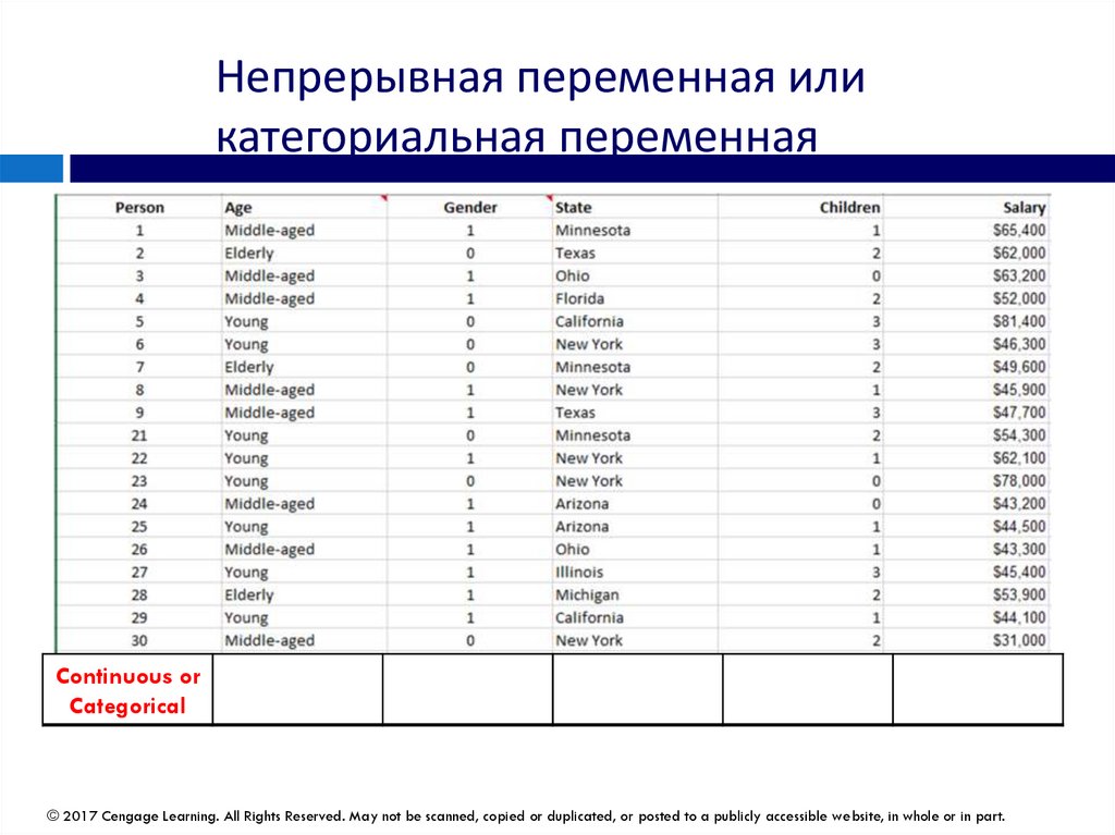
Непрерывная переменная иликатегориальная переменная
Continuous or
Categorical
© 2017 Cengage Learning. All Rights Reserved. May not be scanned, copied or duplicated, or posted to a publicly accessible website, in whole or in part.
30.
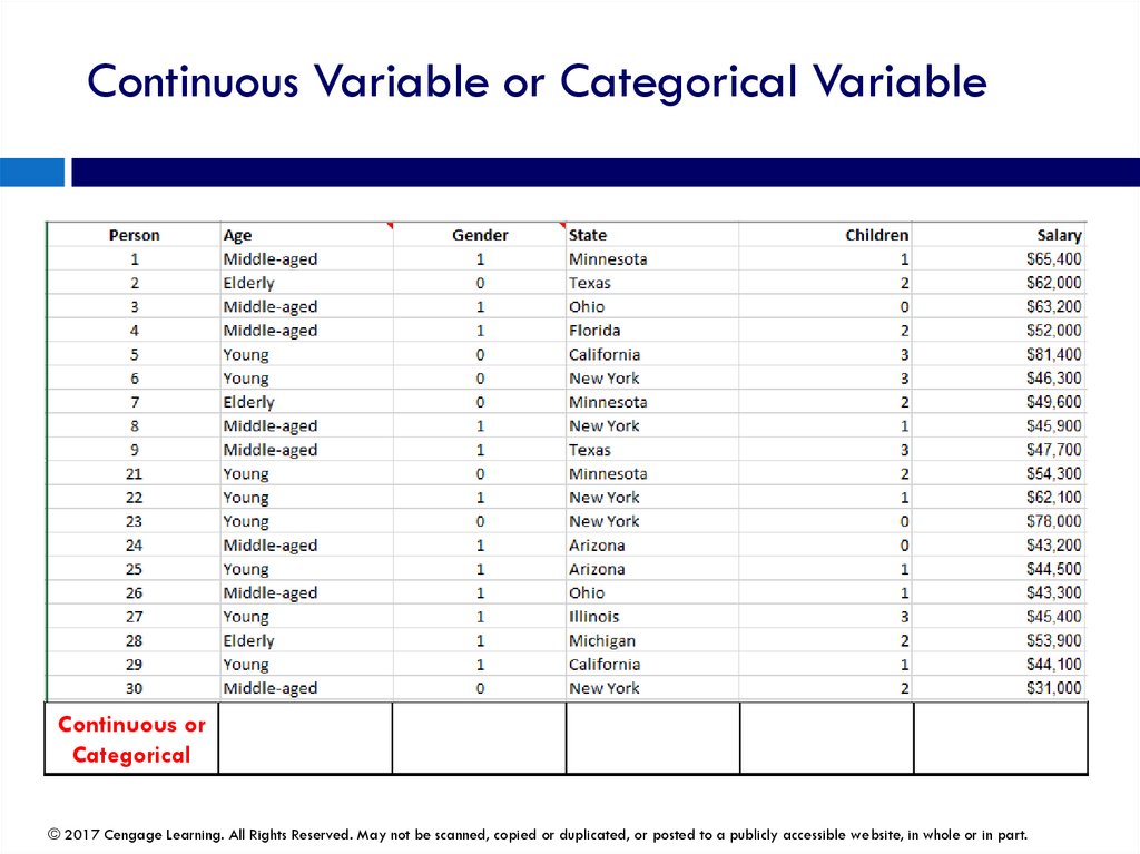
Continuous Variable or Categorical VariableContinuous or
Categorical
© 2017 Cengage Learning. All Rights Reserved. May not be scanned, copied or duplicated, or posted to a publicly accessible website, in whole or in part.
31.
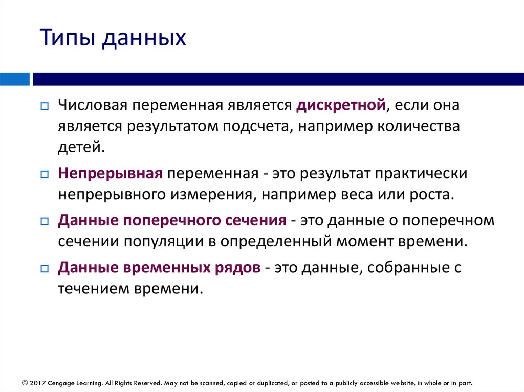
Типы данныхЧисловая переменная является дискретной, если она
является результатом подсчета, например количества
детей.
Непрерывная переменная - это результат практически
непрерывного измерения, например веса или роста.
Данные поперечного сечения - это данные о поперечном
сечении популяции в определенный момент времени.
Данные временных рядов - это данные, собранные с
течением времени.
© 2017 Cengage Learning. All Rights Reserved. May not be scanned, copied or duplicated, or posted to a publicly accessible website, in whole or in part.
32.
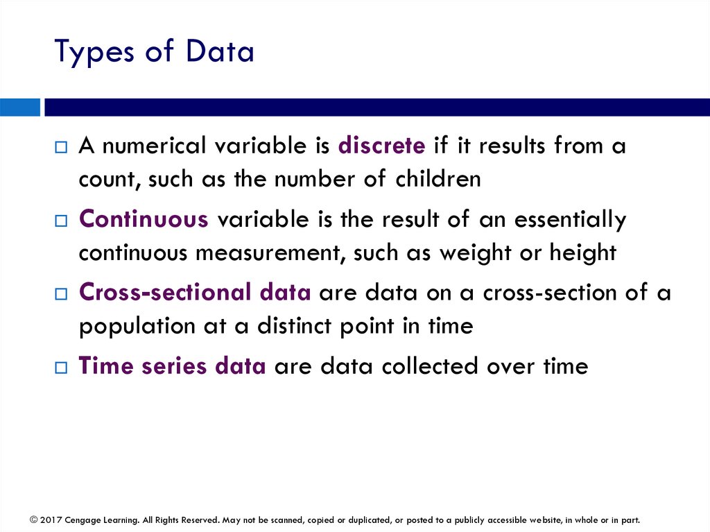
Types of DataA numerical variable is discrete if it results from a
count, such as the number of children
Continuous variable is the result of an essentially
continuous measurement, such as weight or height
Cross-sectional data are data on a cross-section of a
population at a distinct point in time
Time series data are data collected over time
© 2017 Cengage Learning. All Rights Reserved. May not be scanned, copied or duplicated, or posted to a publicly accessible website, in whole or in part.
33.
Типы данных© 2017 Cengage Learning. All Rights Reserved. May not be scanned, copied or duplicated, or posted to a publicly accessible website, in whole or in part.
34.
Types of Data© 2017 Cengage Learning. All Rights Reserved. May not be scanned, copied or duplicated, or posted to a publicly accessible website, in whole or in part.
35.
2-3 Описательные меры для категориальныхпеременны
Есть только несколько возможностей для
описания категориальной переменной, и все
они основаны на подсчете:
Подсчитайте количество категорий
Дайте названия категориям
Подсчитайте количество наблюдений в каждой
категории (итоговые подсчеты могут быть
представлены как «сырые подсчеты» или как
проценты от итоговых значений)
Когда у вас есть счетчики, вы можете отобразить их
графически, обычно в виде столбчатой диаграммы или
круговой диаграммы.
© 2017 Cengage Learning. All Rights Reserved. May not be scanned, copied or duplicated, or posted to a publicly accessible website, in whole or in part.
36.
2-3 Descriptive Measures for Categorical VariablesThere are only a few possibilities for describing a
categorical variable, all based on counting:
Count the number of categories
Give the categories names
Count the number of observations in each category
(The resulting counts can be reported as “raw counts” or
as percentages of totals)
Once you have the counts, you can display them
graphically, usually in a column chart or a pie chart
© 2017 Cengage Learning. All Rights Reserved. May not be scanned, copied or duplicated, or posted to a publicly accessible website, in whole or in part.
37.
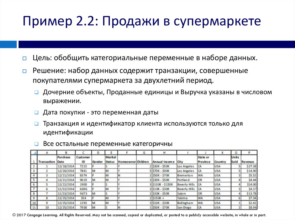
Пример 2.2: Продажи в супермаркетеЦель: обобщить категориальные переменные в наборе данных.
Решение: набор данных содержит транзакции, совершенные
покупателями супермаркета за двухлетний период.
Дочерние объекты, Проданные единицы и Выручка указаны в числовом
выражении.
Дата покупки - это переменная даты
Транзакция и идентификатор клиента используются только для
идентификации
Все остальные переменные категоричны
© 2017 Cengage Learning. All Rights Reserved. May not be scanned, copied or duplicated, or posted to a publicly accessible website, in whole or in part.
38.
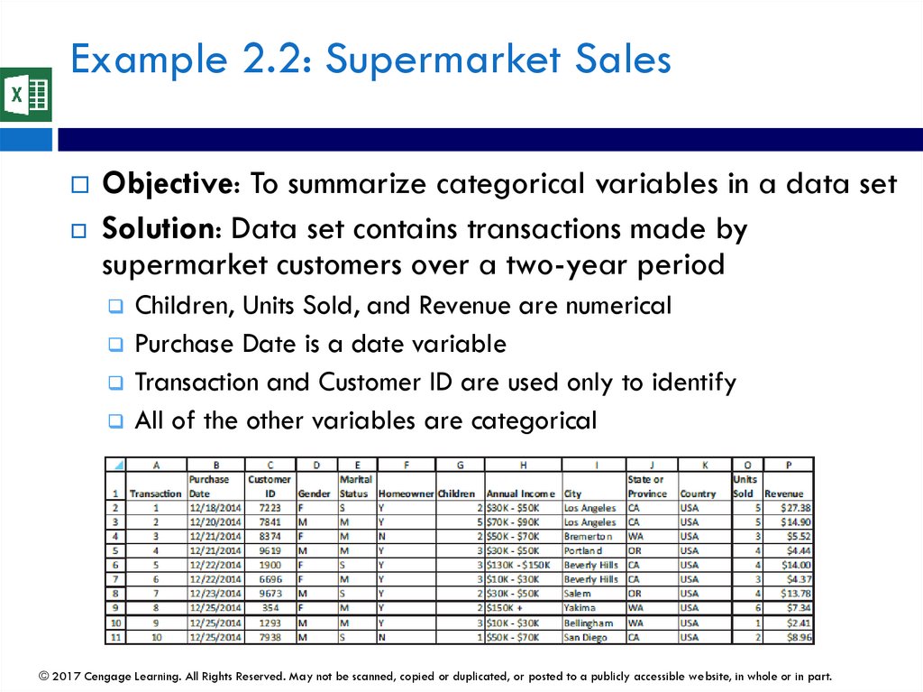
Example 2.2: Supermarket SalesObjective: To summarize categorical variables in a data set
Solution: Data set contains transactions made by
supermarket customers over a two-year period
Children, Units Sold, and Revenue are numerical
Purchase Date is a date variable
Transaction and Customer ID are used only to identify
All of the other variables are categorical
© 2017 Cengage Learning. All Rights Reserved. May not be scanned, copied or duplicated, or posted to a publicly accessible website, in whole or in part.
39.
Пример 2.2: Продажи в супермаркетеЧтобы подсчитать пол, используйте SPSS
Чтобы получить проценты, разделите каждое
количество на общее количество наблюдений.
Делайте диаграммы простыми, чтобы
содержащаяся в них информация отображалась
как можно яснее.
© 2017 Cengage Learning. All Rights Reserved. May not be scanned, copied or duplicated, or posted to a publicly accessible website, in whole or in part.
40.
Example 2.2: Supermarket SalesTo get the counts of Gender, use SPSS
To get the percentages, divide each count by the total
number of observations
Keep charts simple so that the information they contain
emerges as clearly as possible
© 2017 Cengage Learning. All Rights Reserved. May not be scanned, copied or duplicated, or posted to a publicly accessible website, in whole or in part.
41.
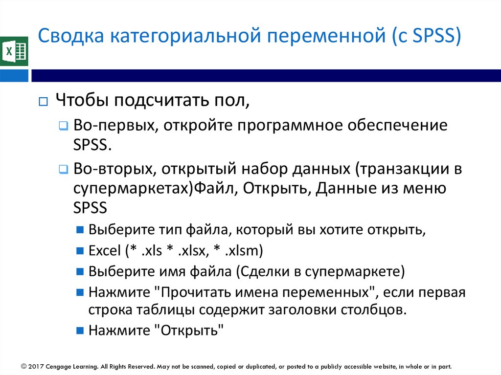
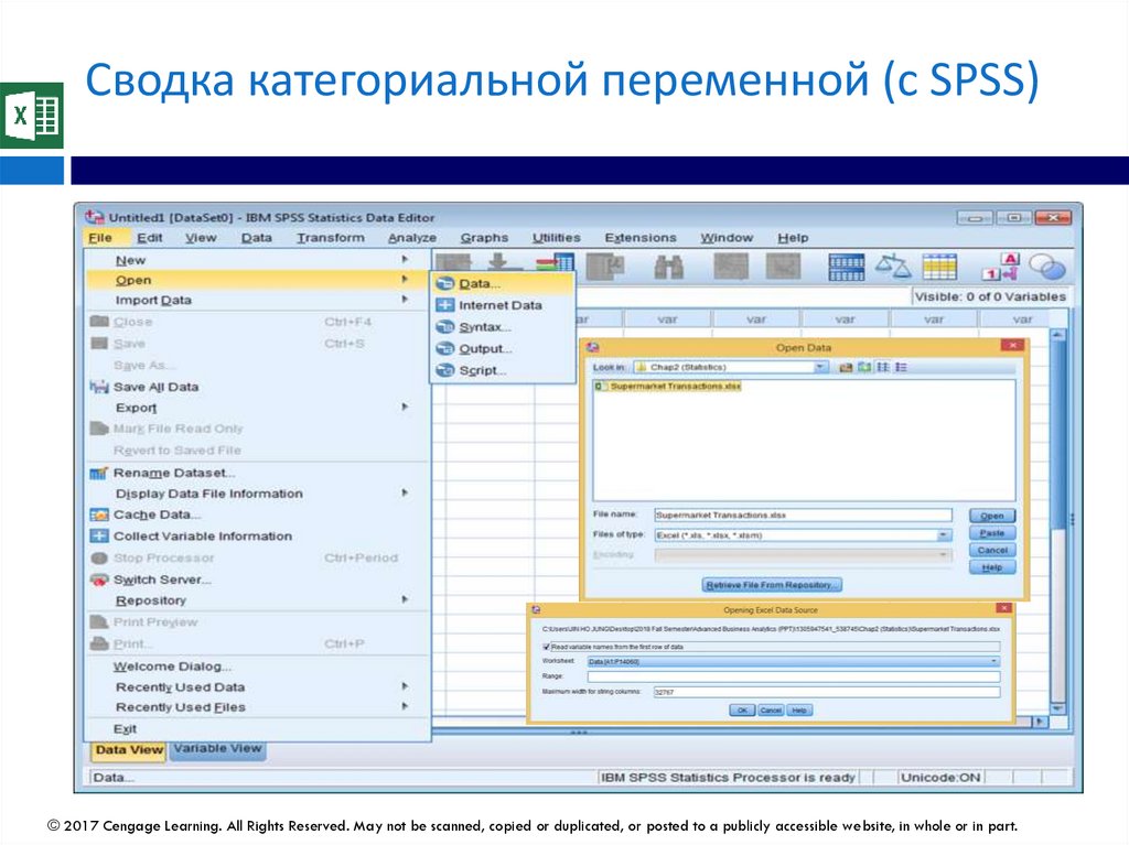
Сводка категориальной переменной (с SPSS)Чтобы подсчитать пол,
Во-первых, откройте программное обеспечение
SPSS.
Во-вторых, открытый набор данных (транзакции в
супермаркетах)Файл, Открыть, Данные из меню
SPSS
Выберите тип файла, который вы хотите открыть,
Excel (* .xls * .xlsx, * .xlsm)
Выберите имя файла (Сделки в супермаркете)
Нажмите "Прочитать имена переменных", если первая
строка таблицы содержит заголовки столбцов.
Нажмите "Открыть"
© 2017 Cengage Learning. All Rights Reserved. May not be scanned, copied or duplicated, or posted to a publicly accessible website, in whole or in part.
42.
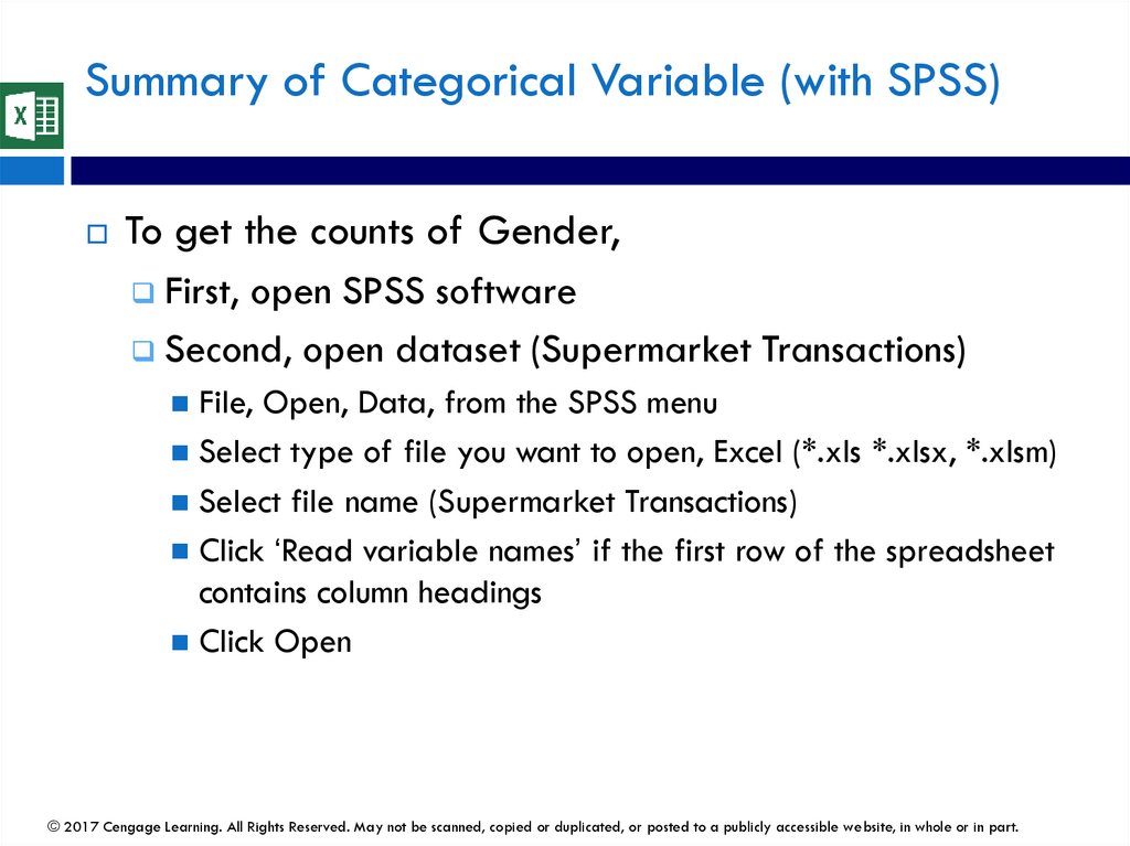
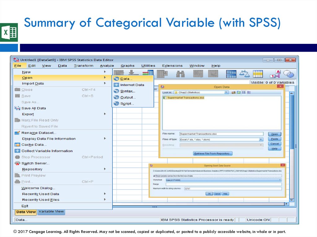
Summary of Categorical Variable (with SPSS)To get the counts of Gender,
First, open SPSS software
Second, open dataset (Supermarket Transactions)
File, Open, Data, from the SPSS menu
Select type of file you want to open, Excel (*.xls *.xlsx, *.xlsm)
Select file name (Supermarket Transactions)
Click ‘Read variable names’ if the first row of the spreadsheet
contains column headings
Click Open
© 2017 Cengage Learning. All Rights Reserved. May not be scanned, copied or duplicated, or posted to a publicly accessible website, in whole or in part.
43.
Сводка категориальной переменной (с SPSS)© 2017 Cengage Learning. All Rights Reserved. May not be scanned, copied or duplicated, or posted to a publicly accessible website, in whole or in part.
44.
Summary of Categorical Variable (with SPSS)© 2017 Cengage Learning. All Rights Reserved. May not be scanned, copied or duplicated, or posted to a publicly accessible website, in whole or in part.
45.
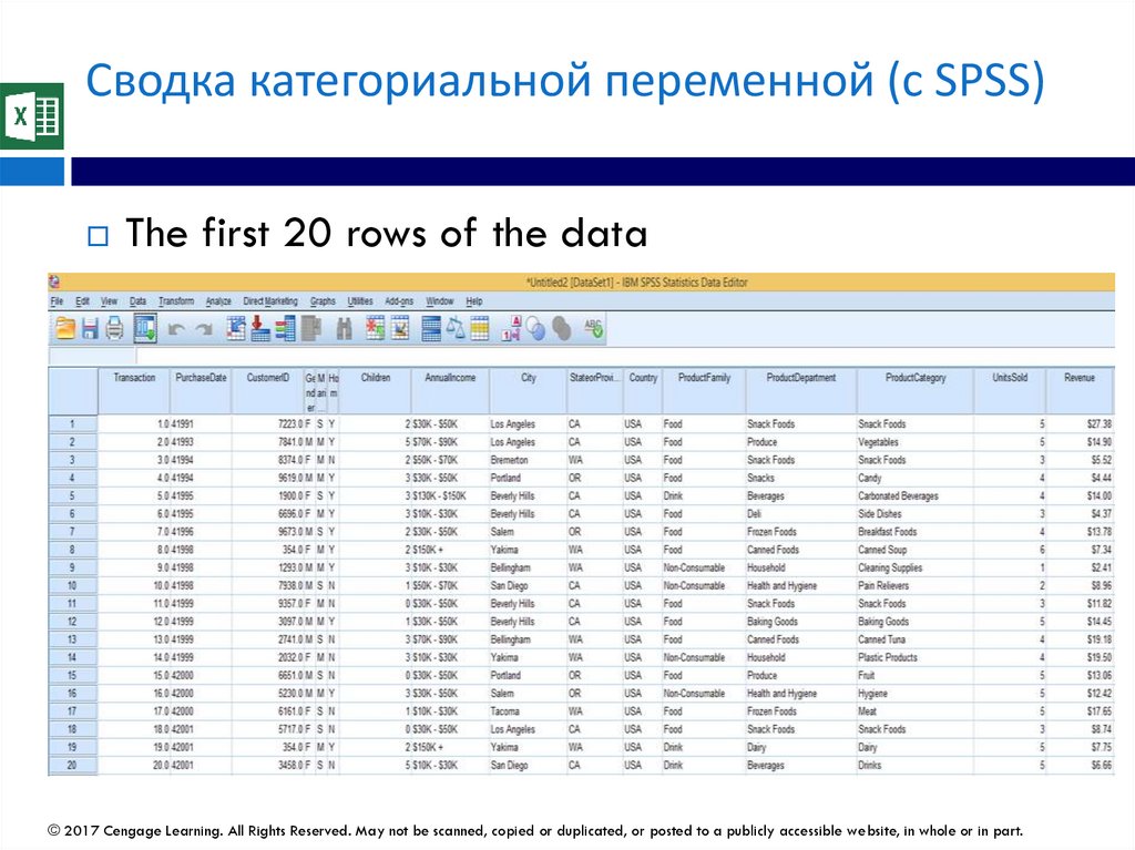
Сводка категориальной переменной (с SPSS)The first 20 rows of the data
© 2017 Cengage Learning. All Rights Reserved. May not be scanned, copied or duplicated, or posted to a publicly accessible website, in whole or in part.
46.
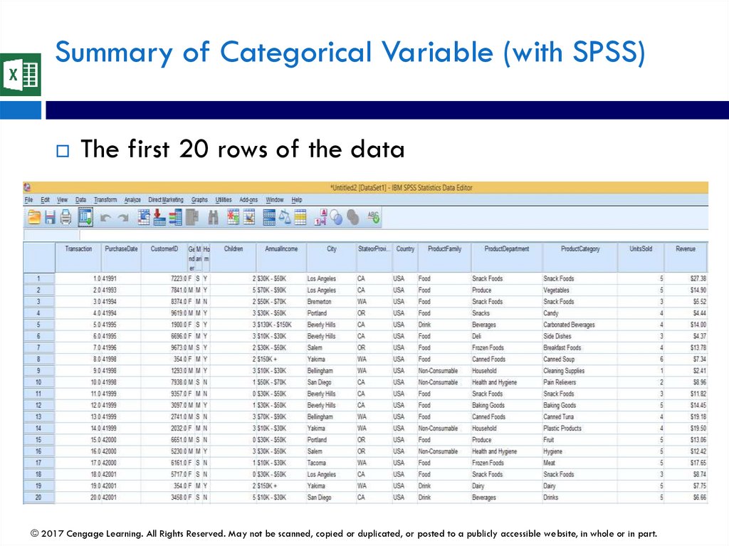
Summary of Categorical Variable (with SPSS)The first 20 rows of the data
© 2017 Cengage Learning. All Rights Reserved. May not be scanned, copied or duplicated, or posted to a publicly accessible website, in whole or in part.
47.
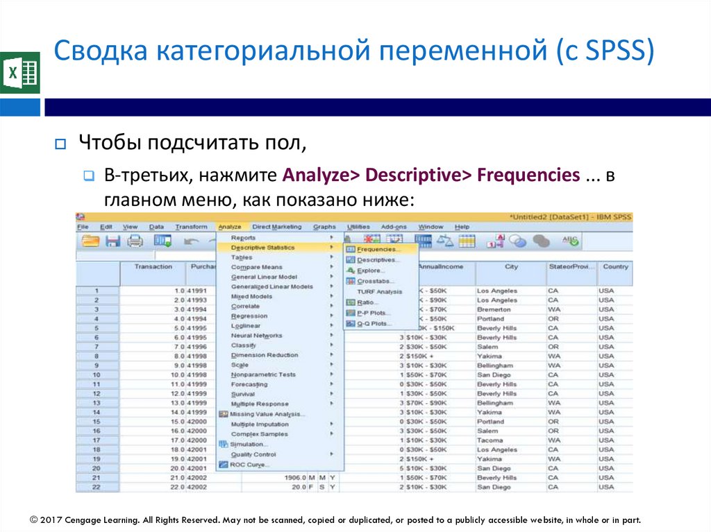
Сводка категориальной переменной (с SPSS)Чтобы подсчитать пол,
В-третьих, нажмите Analyze> Descriptive> Frequencies ... в
главном меню, как показано ниже:
© 2017 Cengage Learning. All Rights Reserved. May not be scanned, copied or duplicated, or posted to a publicly accessible website, in whole or in part.
48.
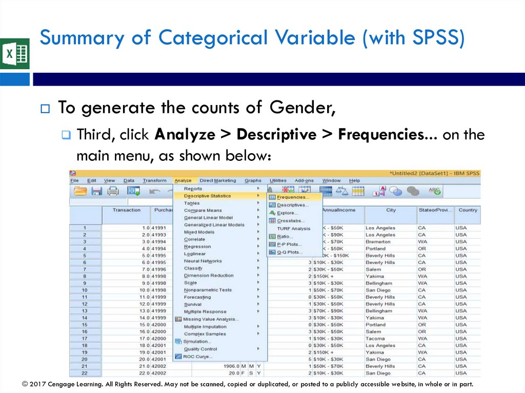
Summary of Categorical Variable (with SPSS)To generate the counts of Gender,
Third, click Analyze > Descriptive > Frequencies... on the
main menu, as shown below:
© 2017 Cengage Learning. All Rights Reserved. May not be scanned, copied or duplicated, or posted to a publicly accessible website, in whole or in part.
49.
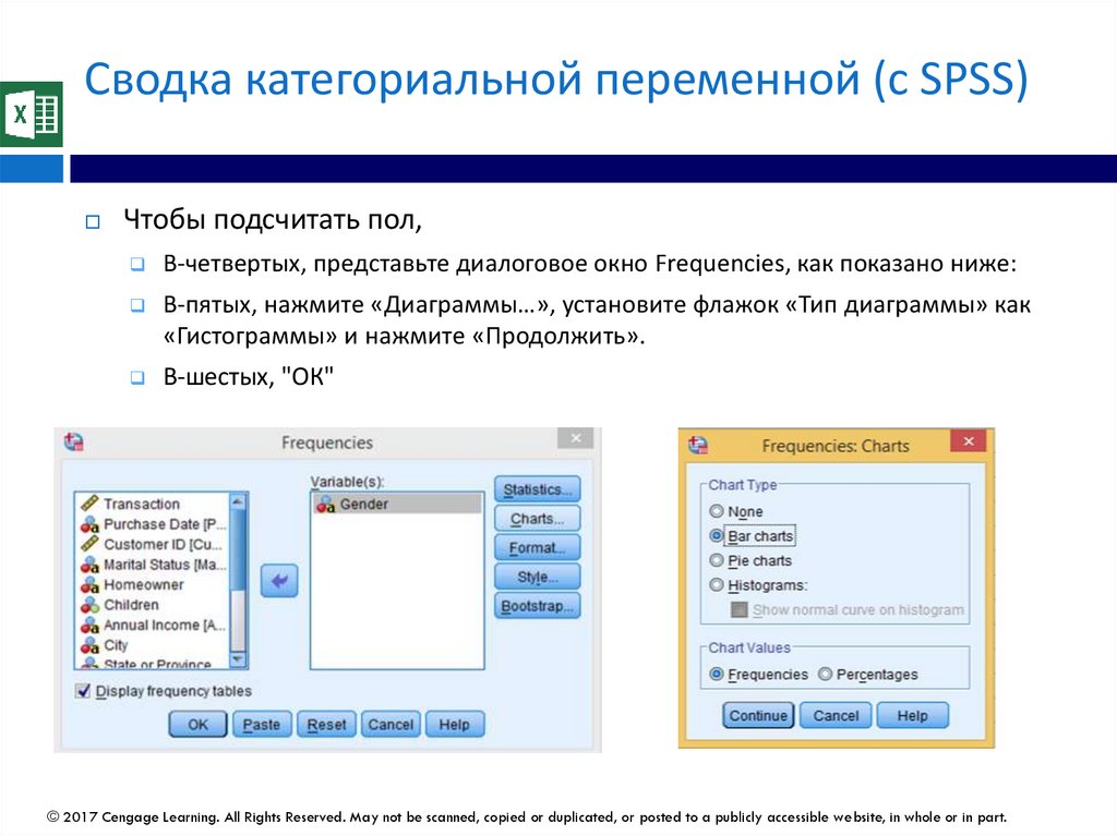
Сводка категориальной переменной (с SPSS)Чтобы подсчитать пол,
В-четвертых, представьте диалоговое окно Frequencies, как показано ниже:
В-пятых, нажмите «Диаграммы…», установите флажок «Тип диаграммы» как
«Гистограммы» и нажмите «Продолжить».
В-шестых, "ОК"
© 2017 Cengage Learning. All Rights Reserved. May not be scanned, copied or duplicated, or posted to a publicly accessible website, in whole or in part.
50.
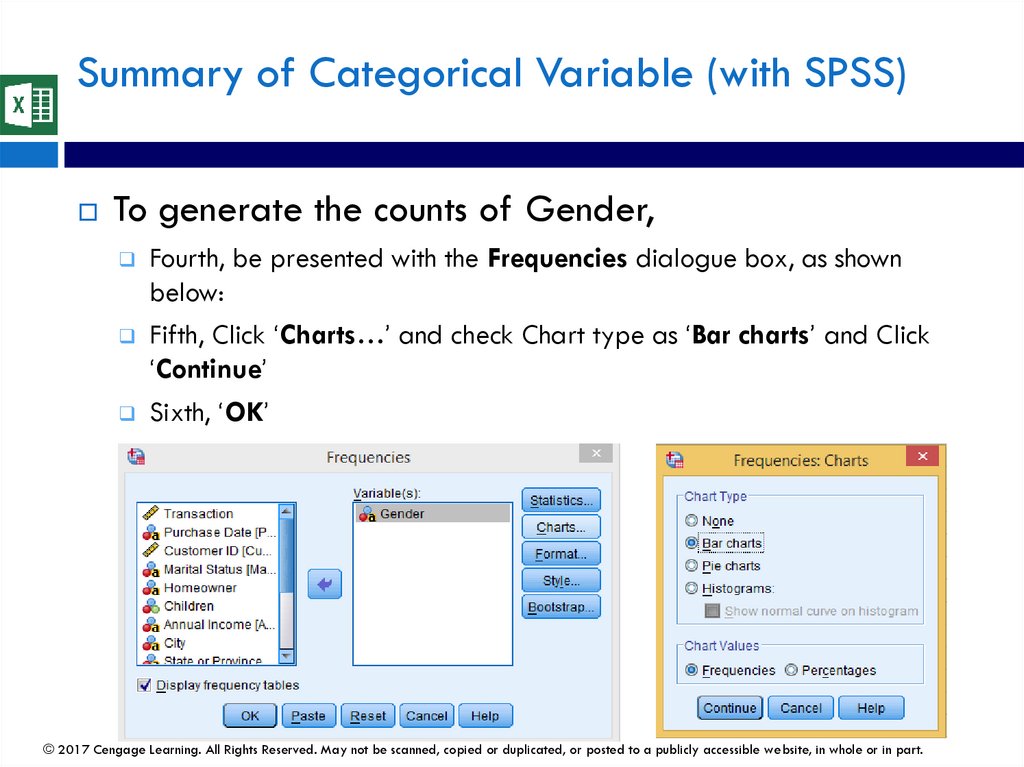
Summary of Categorical Variable (with SPSS)To generate the counts of Gender,
Fourth, be presented with the Frequencies dialogue box, as shown
below:
Fifth, Click ‘Charts…’ and check Chart type as ‘Bar charts’ and Click
‘Continue’
Sixth, ‘OK’
© 2017 Cengage Learning. All Rights Reserved. May not be scanned, copied or duplicated, or posted to a publicly accessible website, in whole or in part.
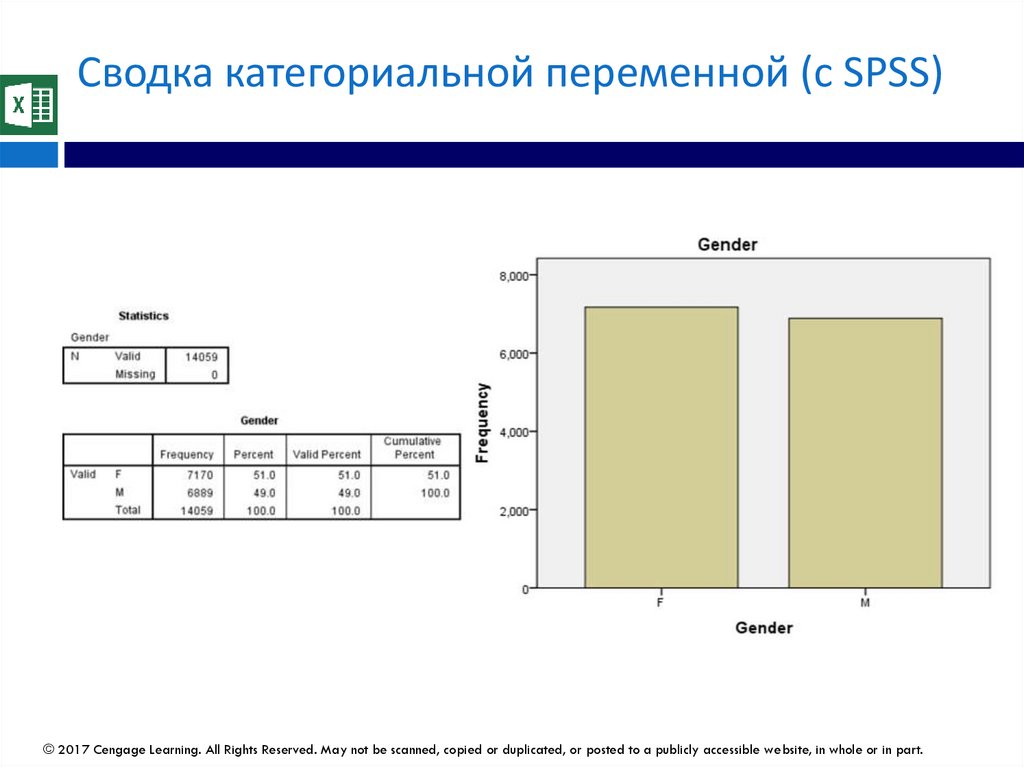
51.
Сводка категориальной переменной (с SPSS)© 2017 Cengage Learning. All Rights Reserved. May not be scanned, copied or duplicated, or posted to a publicly accessible website, in whole or in part.
52.
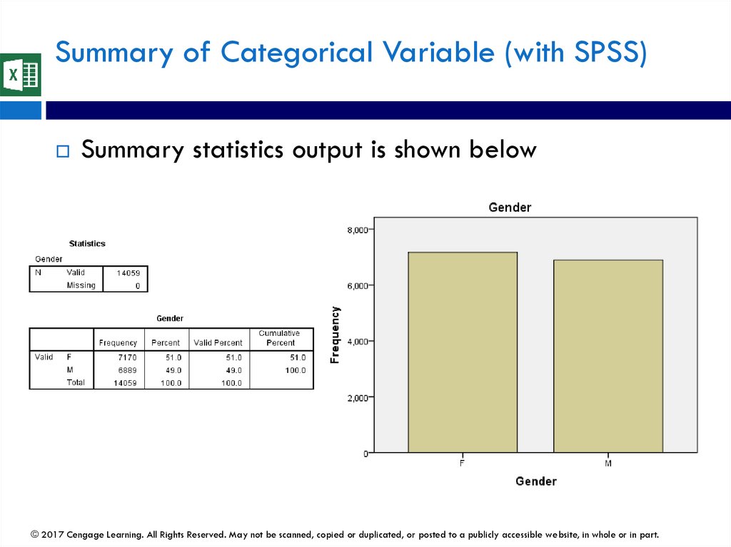
Summary of Categorical Variable (with SPSS)Summary statistics output is shown below
© 2017 Cengage Learning. All Rights Reserved. May not be scanned, copied or duplicated, or posted to a publicly accessible website, in whole or in part.
53.
Классное упражнениеСгенерируйте количество переменных
«MaritalStatus» и «Homeowner».
Создайте гистограммы двух переменных
© 2017 Cengage Learning. All Rights Reserved. May not be scanned, copied or duplicated, or posted to a publicly accessible website, in whole or in part.
54.
Class ExerciseGenerate the counts of ‘MaritalStatus’ and
‘Homeowner’ variables
Generate bar charts of the two variables
© 2017 Cengage Learning. All Rights Reserved. May not be scanned, copied or duplicated, or posted to a publicly accessible website, in whole or in part.
55.
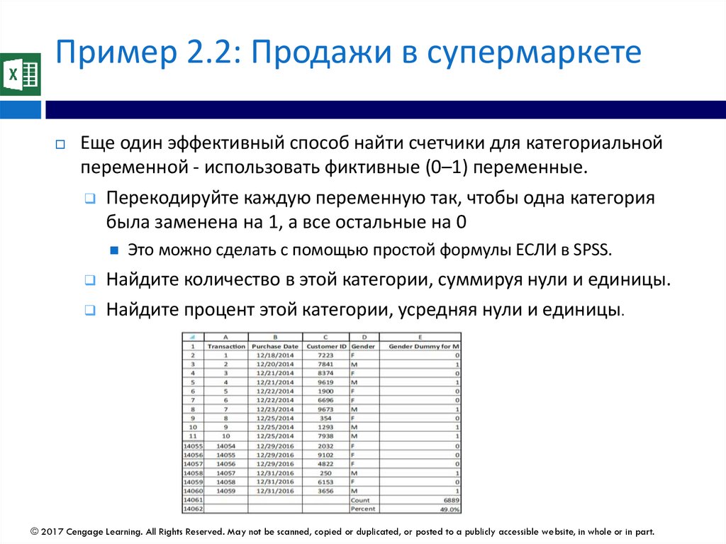
Пример 2.2: Продажи в супермаркетеЕще один эффективный способ найти счетчики для категориальной
переменной - использовать фиктивные (0–1) переменные.
Перекодируйте каждую переменную так, чтобы одна категория
была заменена на 1, а все остальные на 0
Это можно сделать с помощью простой формулы ЕСЛИ в SPSS.
Найдите количество в этой категории, суммируя нули и единицы.
Найдите процент этой категории, усредняя нули и единицы.
© 2017 Cengage Learning. All Rights Reserved. May not be scanned, copied or duplicated, or posted to a publicly accessible website, in whole or in part.
56.
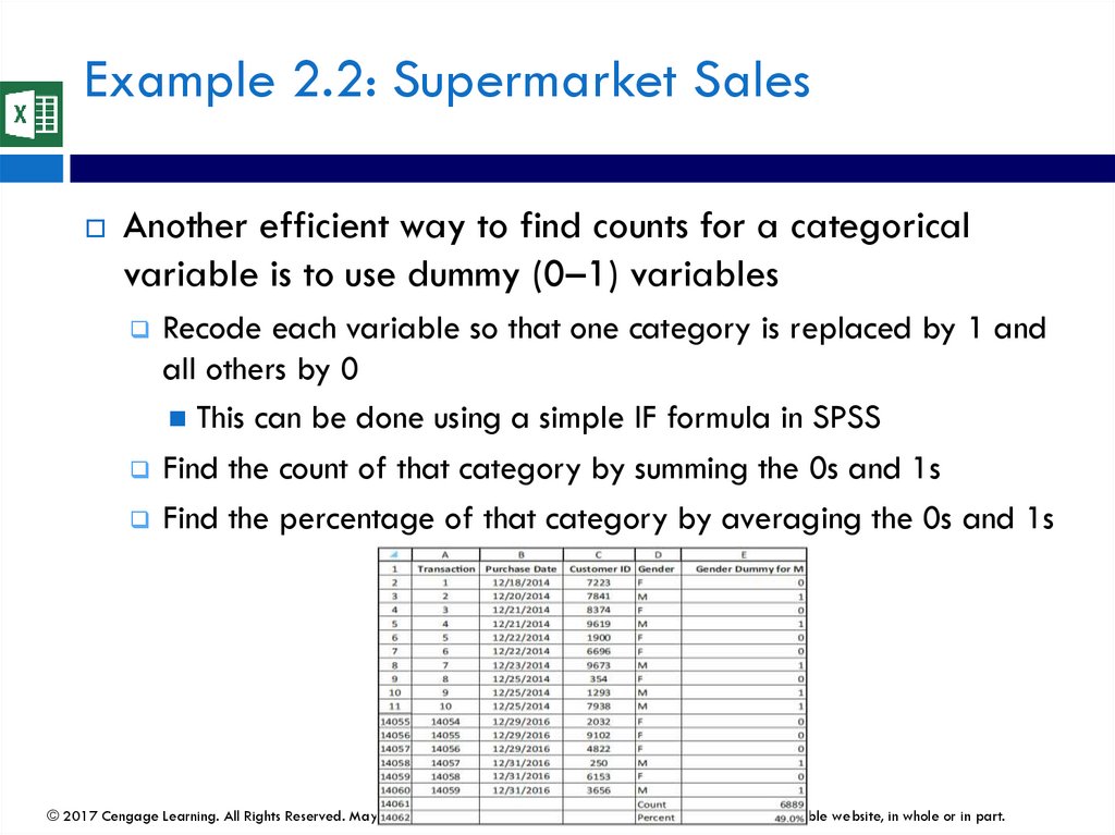
Example 2.2: Supermarket SalesAnother efficient way to find counts for a categorical
variable is to use dummy (0–1) variables
Recode each variable so that one category is replaced by 1 and
all others by 0
This can be done using a simple IF formula in SPSS
Find the count of that category by summing the 0s and 1s
Find the percentage of that category by averaging the 0s and 1s
© 2017 Cengage Learning. All Rights Reserved. May not be scanned, copied or duplicated, or posted to a publicly accessible website, in whole or in part.
57.
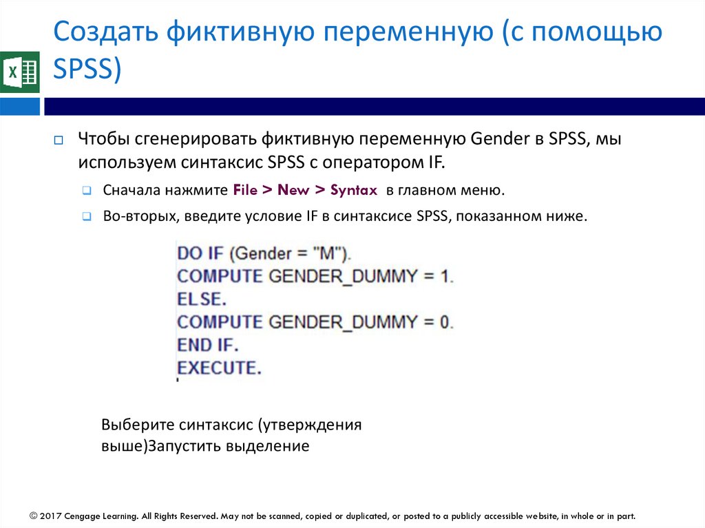
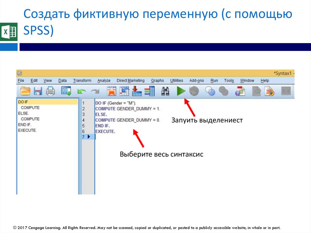
Создать фиктивную переменную (с помощьюSPSS)
Чтобы сгенерировать фиктивную переменную Gender в SPSS, мы
используем синтаксис SPSS с оператором IF.
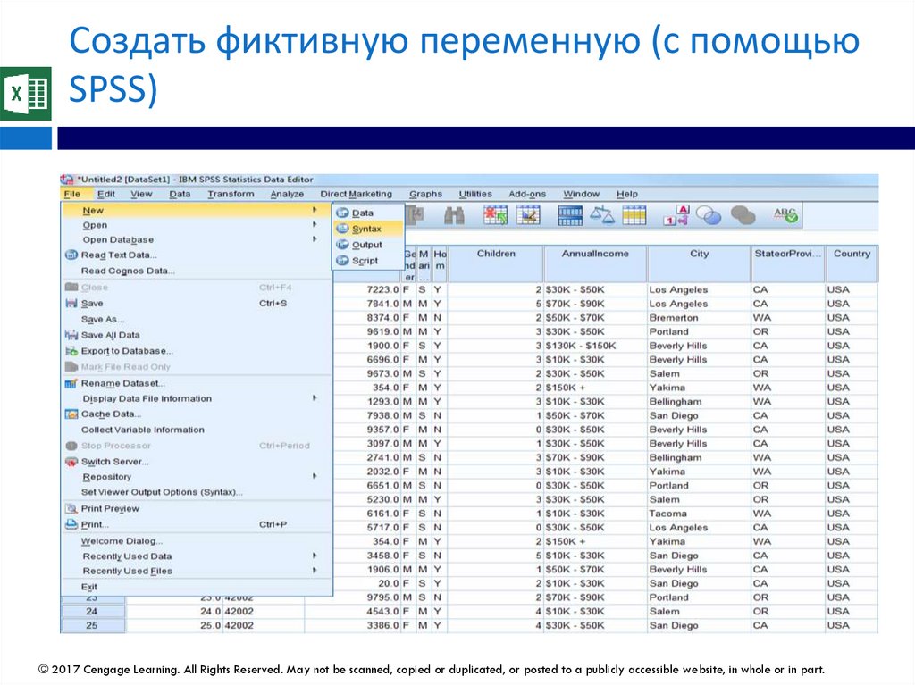
Сначала нажмите File > New > Syntax в главном меню.
Во-вторых, введите условие IF в синтаксисе SPSS, показанном ниже.
Выберите синтаксис (утверждения
выше)Запустить выделение
© 2017 Cengage Learning. All Rights Reserved. May not be scanned, copied or duplicated, or posted to a publicly accessible website, in whole or in part.
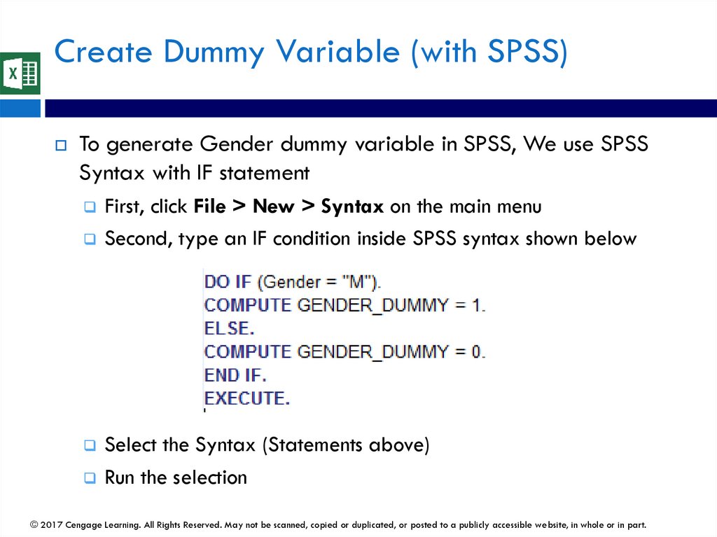
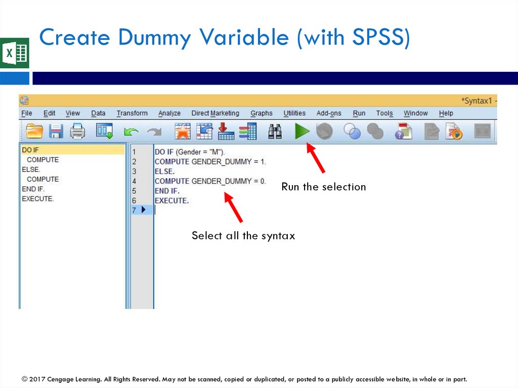
58.
Create Dummy Variable (with SPSS)To generate Gender dummy variable in SPSS, We use SPSS
Syntax with IF statement
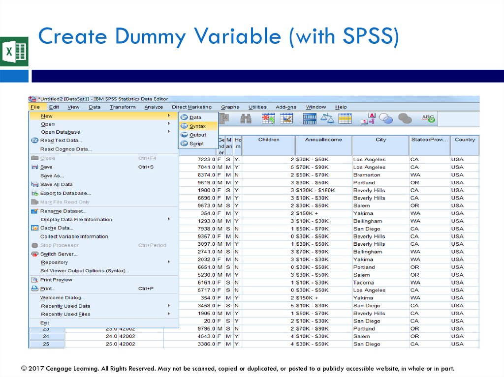
First, click File > New > Syntax on the main menu
Second, type an IF condition inside SPSS syntax shown below
Select the Syntax (Statements above)
Run the selection
© 2017 Cengage Learning. All Rights Reserved. May not be scanned, copied or duplicated, or posted to a publicly accessible website, in whole or in part.
59.
Создать фиктивную переменную (с помощьюSPSS)
© 2017 Cengage Learning. All Rights Reserved. May not be scanned, copied or duplicated, or posted to a publicly accessible website, in whole or in part.
60.
Create Dummy Variable (with SPSS)© 2017 Cengage Learning. All Rights Reserved. May not be scanned, copied or duplicated, or posted to a publicly accessible website, in whole or in part.
61.
Создать фиктивную переменную (с помощьюSPSS)
Запуить выделениест
Выберите весь синтаксис
© 2017 Cengage Learning. All Rights Reserved. May not be scanned, copied or duplicated, or posted to a publicly accessible website, in whole or in part.
62.
Create Dummy Variable (with SPSS)Run the selection
Select all the syntax
© 2017 Cengage Learning. All Rights Reserved. May not be scanned, copied or duplicated, or posted to a publicly accessible website, in whole or in part.
63.
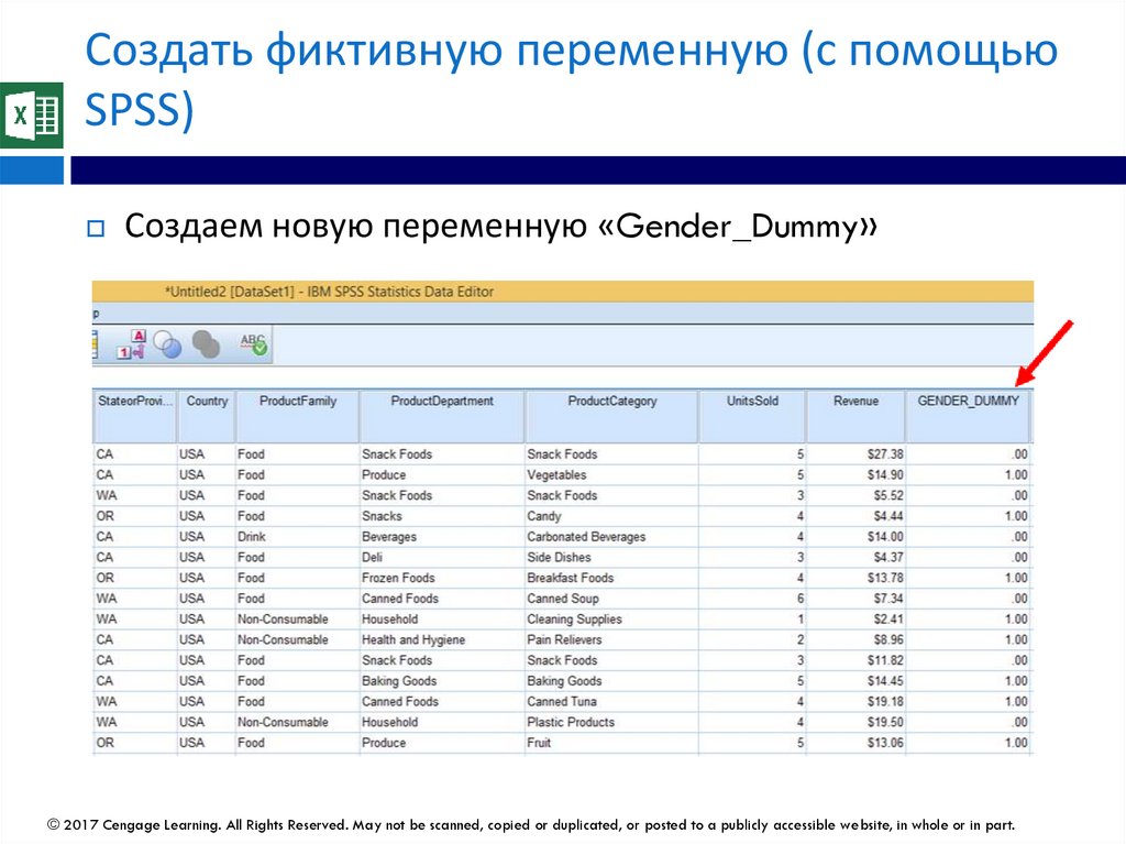
Создать фиктивную переменную (с помощьюSPSS)
Создаем новую переменную «Gender_Dummy»
© 2017 Cengage Learning. All Rights Reserved. May not be scanned, copied or duplicated, or posted to a publicly accessible website, in whole or in part.
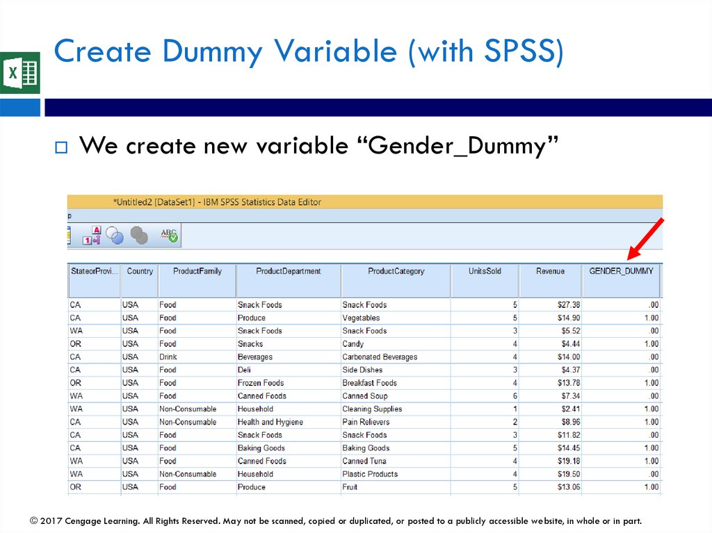
64.
Create Dummy Variable (with SPSS)We create new variable “Gender_Dummy”
© 2017 Cengage Learning. All Rights Reserved. May not be scanned, copied or duplicated, or posted to a publicly accessible website, in whole or in part.
65.
Классное упражнениеПожалуйста, создайте новую фиктивную
переменную MaritalStatus
Назовите фиктивную переменную MS_Dummy
Замените S на 0 в MS_Dummy
Замените M на 1 в MS_Dummy
© 2017 Cengage Learning. All Rights Reserved. May not be scanned, copied or duplicated, or posted to a publicly accessible website, in whole or in part.
66.
Class ExercisePlease create new dummy variable of MaritalStatus
Name the dummy variable as MS_Dummy
Replace S with 0 in MS_Dummy
Replace M with 1 in MS_Dummy
© 2017 Cengage Learning. All Rights Reserved. May not be scanned, copied or duplicated, or posted to a publicly accessible website, in whole or in part.
67.
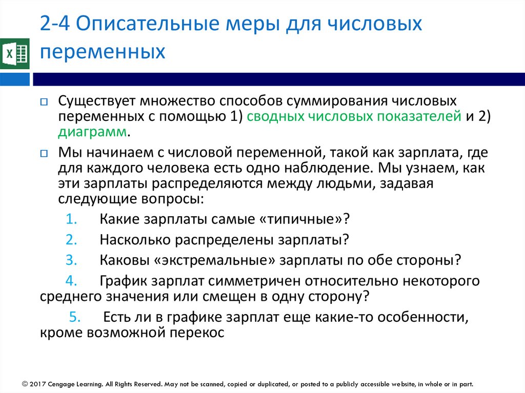
2-4 Описательные меры для числовыхпеременных
Существует множество способов суммирования числовых
переменных с помощью 1) сводных числовых показателей и 2)
диаграмм.
Мы начинаем с числовой переменной, такой как зарплата, где
для каждого человека есть одно наблюдение. Мы узнаем, как
эти зарплаты распределяются между людьми, задавая
следующие вопросы:
1. Какие зарплаты самые «типичные»?
2. Насколько распределены зарплаты?
3. Каковы «экстремальные» зарплаты по обе стороны?
4. График зарплат симметричен относительно некоторого
среднего значения или смещен в одну сторону?
5. Есть ли в графике зарплат еще какие-то особенности,
кроме возможной перекос
© 2017 Cengage Learning. All Rights Reserved. May not be scanned, copied or duplicated, or posted to a publicly accessible website, in whole or in part.
68.
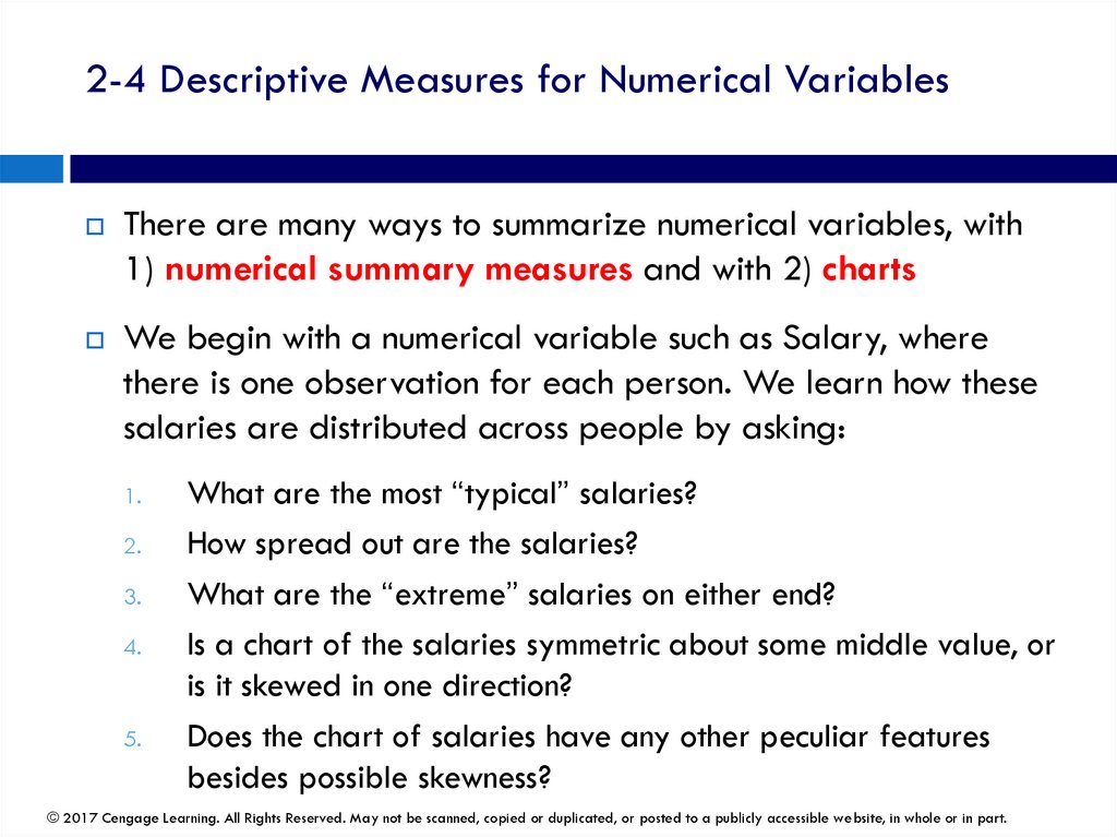
2-4 Descriptive Measures for Numerical VariablesThere are many ways to summarize numerical variables, with
1) numerical summary measures and with 2) charts
We begin with a numerical variable such as Salary, where
there is one observation for each person. We learn how these
salaries are distributed across people by asking:
1.
2.
3.
4.
5.
What are the most “typical” salaries?
How spread out are the salaries?
What are the “extreme” salaries on either end?
Is a chart of the salaries symmetric about some middle value, or
is it skewed in one direction?
Does the chart of salaries have any other peculiar features
besides possible skewness?
© 2017 Cengage Learning. All Rights Reserved. May not be scanned, copied or duplicated, or posted to a publicly accessible website, in whole or in part.
69.
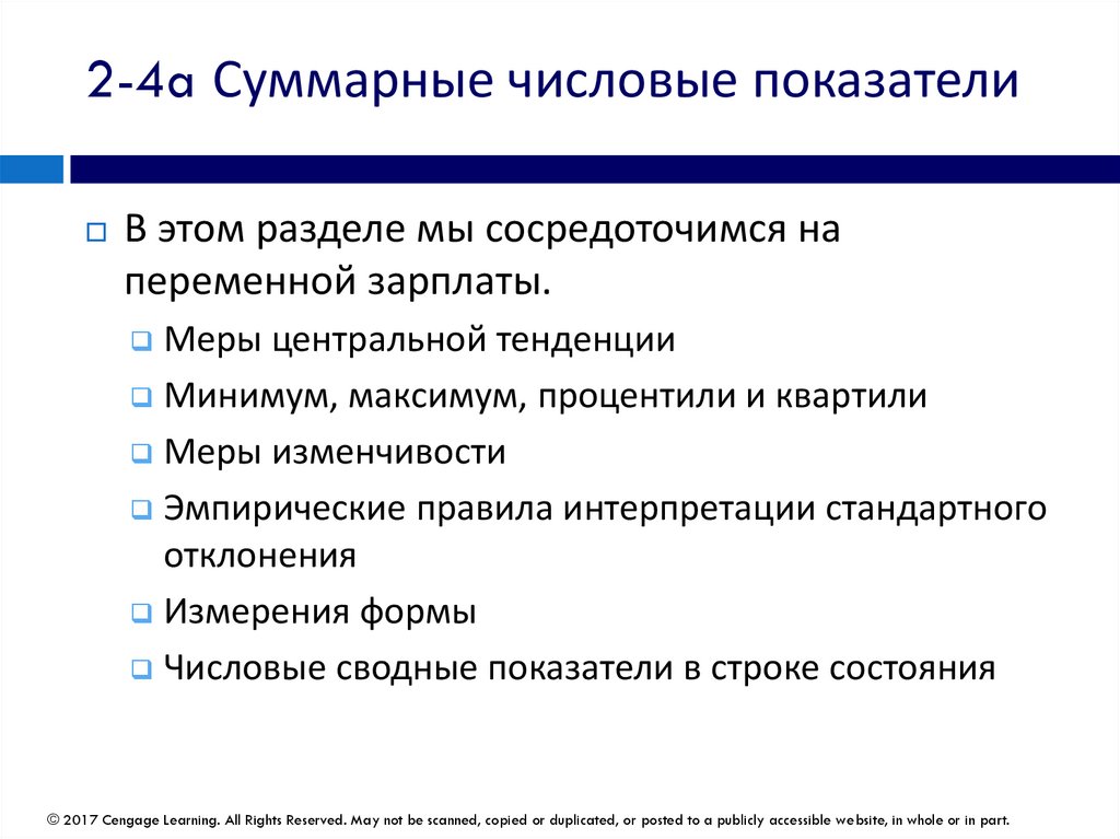
2-4a Суммарные числовые показателиВ этом разделе мы сосредоточимся на
переменной зарплаты.
Меры центральной тенденции
Минимум, максимум, процентили и квартили
Меры изменчивости
Эмпирические правила интерпретации стандартного
отклонения
Измерения формы
Числовые сводные показатели в строке состояния
© 2017 Cengage Learning. All Rights Reserved. May not be scanned, copied or duplicated, or posted to a publicly accessible website, in whole or in part.
70.
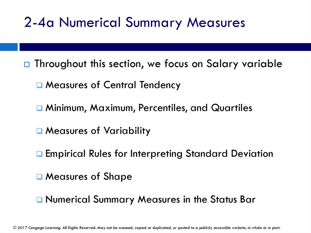
2-4a Numerical Summary MeasuresThroughout this section, we focus on Salary variable
Measures of Central Tendency
Minimum, Maximum, Percentiles, and Quartiles
Measures of Variability
Empirical Rules for Interpreting Standard Deviation
Measures of Shape
Numerical Summary Measures in the Status Bar
© 2017 Cengage Learning. All Rights Reserved. May not be scanned, copied or duplicated, or posted to a publicly accessible website, in whole or in part.
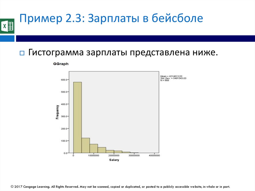
71.
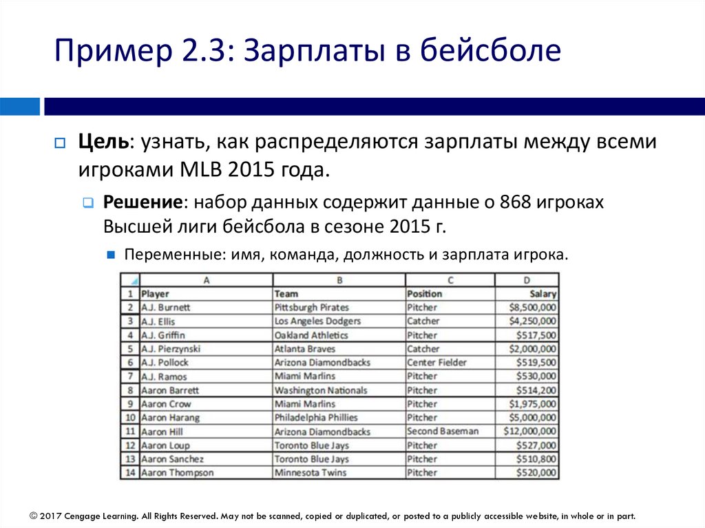
Пример 2.3: Зарплаты в бейсболеЦель: узнать, как распределяются зарплаты между всеми
игроками MLB 2015 года.
Решение: набор данных содержит данные о 868 игроках
Высшей лиги бейсбола в сезоне 2015 г.
Переменные: имя, команда, должность и зарплата игрока.
© 2017 Cengage Learning. All Rights Reserved. May not be scanned, copied or duplicated, or posted to a publicly accessible website, in whole or in part.
72.
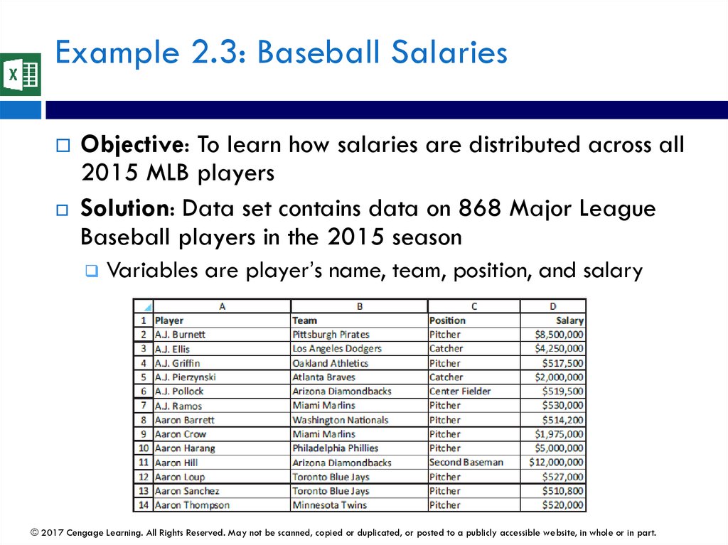
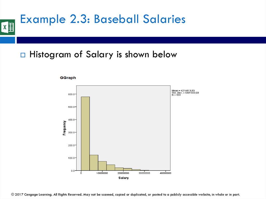
Example 2.3: Baseball SalariesObjective: To learn how salaries are distributed across all
2015 MLB players
Solution: Data set contains data on 868 Major League
Baseball players in the 2015 season
Variables are player’s name, team, position, and salary
© 2017 Cengage Learning. All Rights Reserved. May not be scanned, copied or duplicated, or posted to a publicly accessible website, in whole or in part.
73.
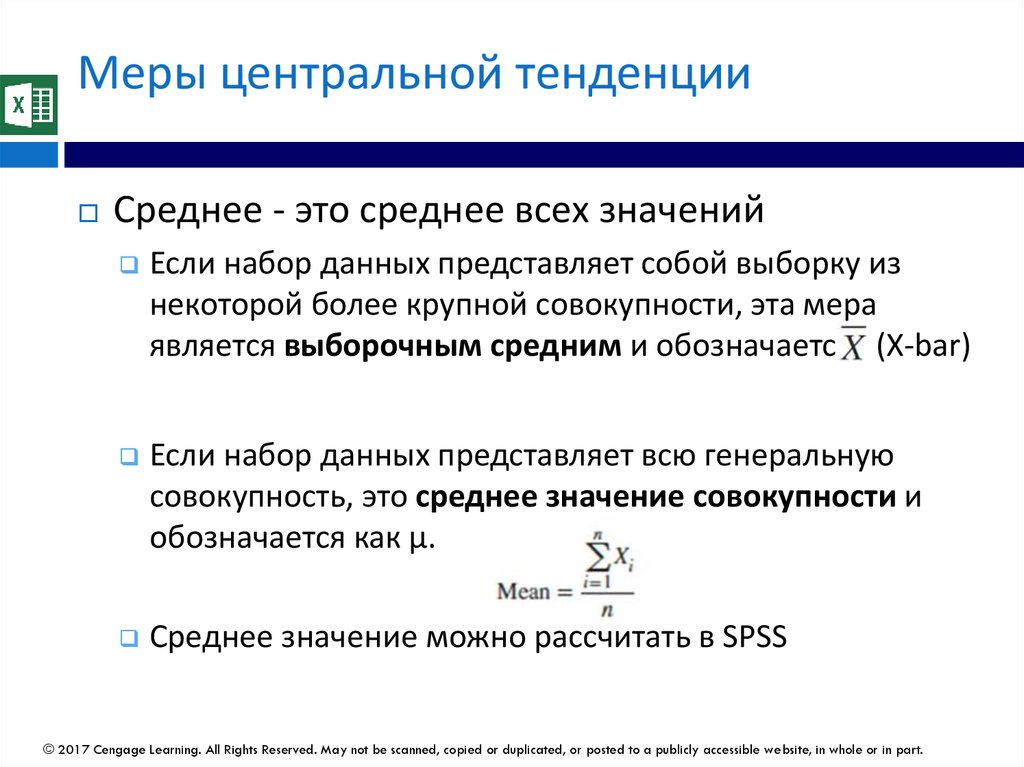
Меры центральной тенденцииСреднее - это среднее всех значений
Если набор данных представляет собой выборку из
некоторой более крупной совокупности, эта мера
является выборочным средним и обозначается (X-bar)
Если набор данных представляет всю генеральную
совокупность, это среднее значение совокупности и
обозначается как μ.
Среднее значение можно рассчитать в SPSS
© 2017 Cengage Learning. All Rights Reserved. May not be scanned, copied or duplicated, or posted to a publicly accessible website, in whole or in part.
74.
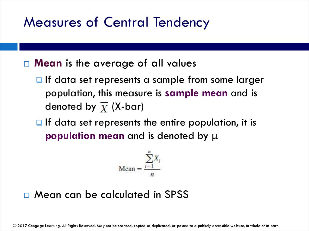
Measures of Central TendencyMean is the average of all values
If data set represents a sample from some larger
population, this measure is sample mean and is
denoted by (X-bar)
If data set represents the entire population, it is
population mean and is denoted by μ
Mean can be calculated in SPSS
© 2017 Cengage Learning. All Rights Reserved. May not be scanned, copied or duplicated, or posted to a publicly accessible website, in whole or in part.
75.
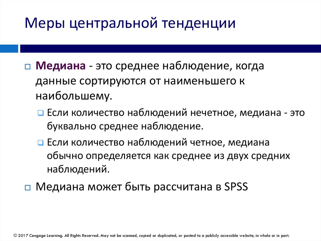
Меры центральной тенденцииМедиана - это среднее наблюдение, когда
данные сортируются от наименьшего к
наибольшему.
Если количество наблюдений нечетное, медиана - это
буквально среднее наблюдение.
Если количество наблюдений четное, медиана
обычно определяется как среднее из двух средних
наблюдений.
Медиана может быть рассчитана в SPSS
© 2017 Cengage Learning. All Rights Reserved. May not be scanned, copied or duplicated, or posted to a publicly accessible website, in whole or in part.
76.
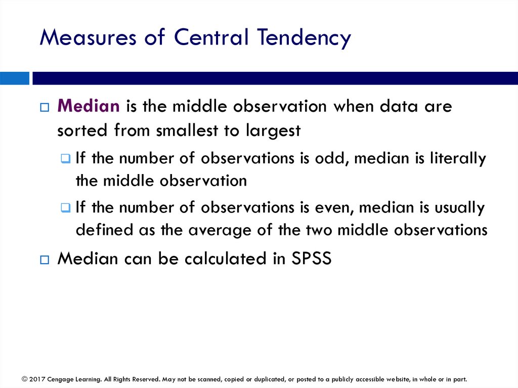
Measures of Central TendencyMedian is the middle observation when data are
sorted from smallest to largest
If the number of observations is odd, median is literally
the middle observation
If the number of observations is even, median is usually
defined as the average of the two middle observations
Median can be calculated in SPSS
© 2017 Cengage Learning. All Rights Reserved. May not be scanned, copied or duplicated, or posted to a publicly accessible website, in whole or in part.
77.
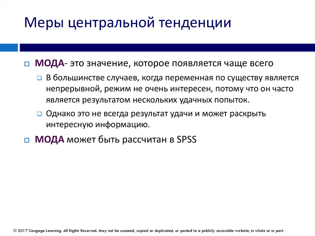
Меры центральной тенденцииМОДА- это значение, которое появляется чаще всего
В большинстве случаев, когда переменная по существу является
непрерывной, режим не очень интересен, потому что он часто
является результатом нескольких удачных попыток.
Однако это не всегда результат удачи и может раскрыть
интересную информацию.
МОДА может быть рассчитан в SPSS
© 2017 Cengage Learning. All Rights Reserved. May not be scanned, copied or duplicated, or posted to a publicly accessible website, in whole or in part.
78.
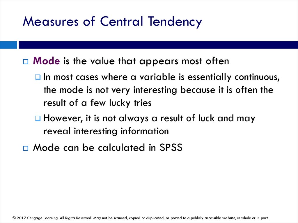
Measures of Central TendencyMode is the value that appears most often
In most cases where a variable is essentially continuous,
the mode is not very interesting because it is often the
result of a few lucky tries
However, it is not always a result of luck and may
reveal interesting information
Mode can be calculated in SPSS
© 2017 Cengage Learning. All Rights Reserved. May not be scanned, copied or duplicated, or posted to a publicly accessible website, in whole or in part.
79.
Пример 2.3: Зарплаты в бейсболе© 2017 Cengage Learning. All Rights Reserved. May not be scanned, copied or duplicated, or posted to a publicly accessible website, in whole or in part.
80.
Example 2.3: Baseball Salaries© 2017 Cengage Learning. All Rights Reserved. May not be scanned, copied or duplicated, or posted to a publicly accessible website, in whole or in part.
81.
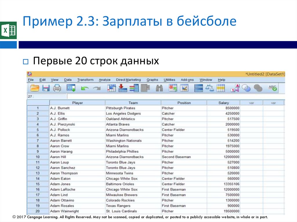
Пример 2.3: Зарплаты в бейсболеПервые 20 строк данных
© 2017 Cengage Learning. All Rights Reserved. May not be scanned, copied or duplicated, or posted to a publicly accessible website, in whole or in part.
82.
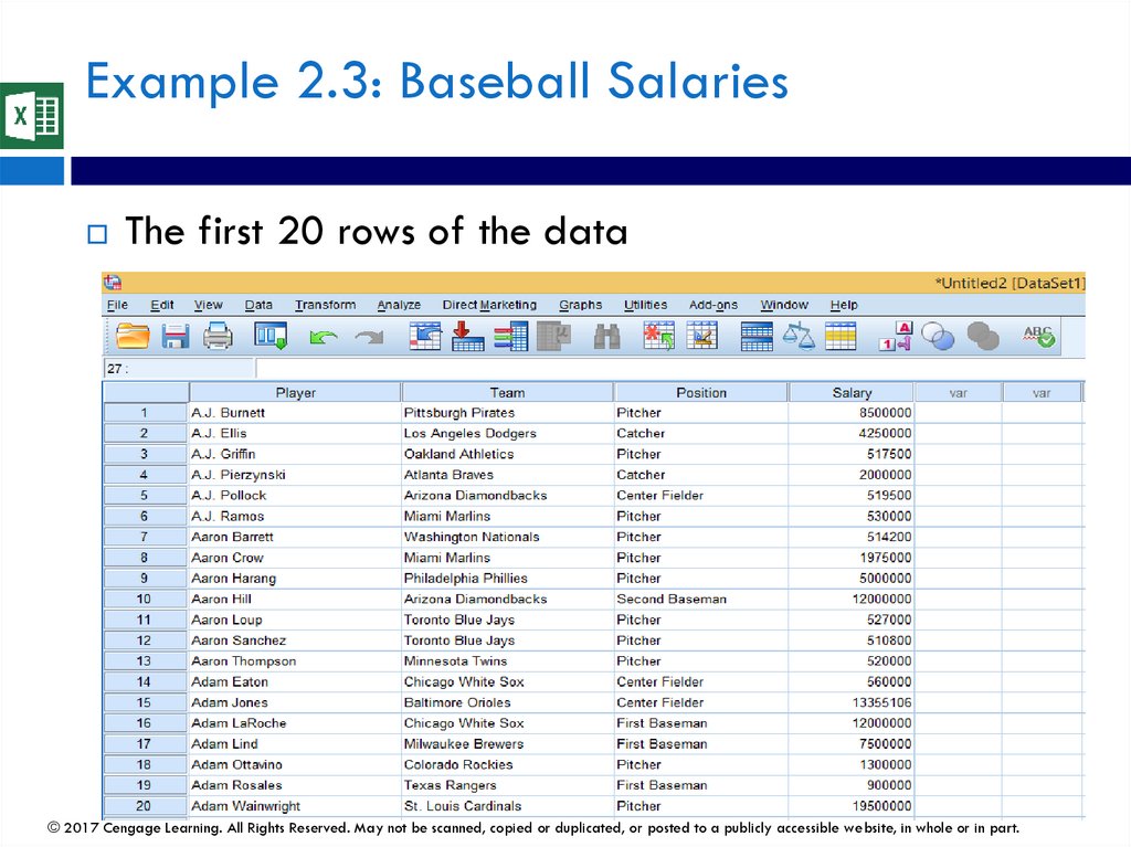
Example 2.3: Baseball SalariesThe first 20 rows of the data
© 2017 Cengage Learning. All Rights Reserved. May not be scanned, copied or duplicated, or posted to a publicly accessible website, in whole or in part.
83.
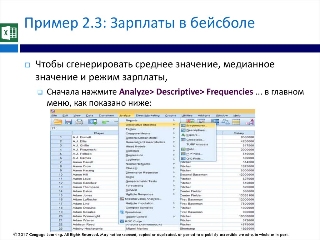
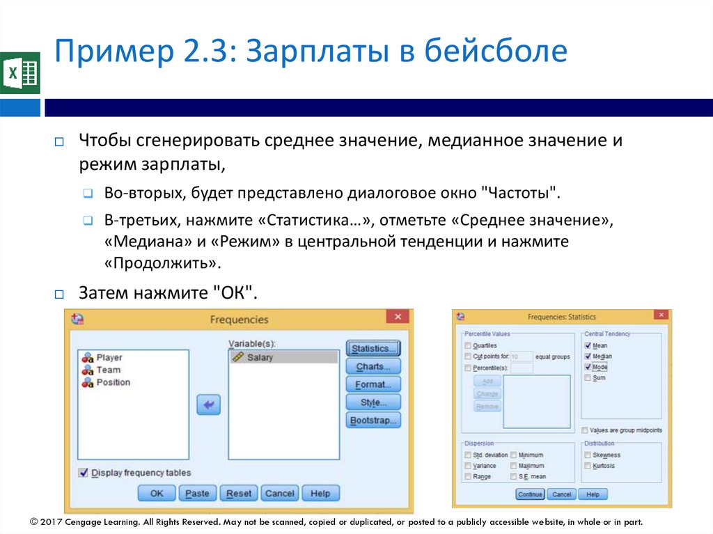
Пример 2.3: Зарплаты в бейсболеЧтобы сгенерировать среднее значение, медианное
значение и режим зарплаты,
Сначала нажмите Analyze> Descriptive> Frequencies ... в главном
меню, как показано ниже:
© 2017 Cengage Learning. All Rights Reserved. May not be scanned, copied or duplicated, or posted to a publicly accessible website, in whole or in part.
84.
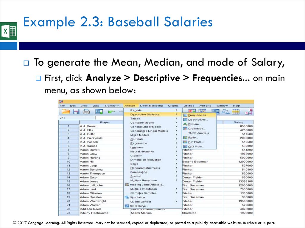
Example 2.3: Baseball SalariesTo generate the Mean, Median, and mode of Salary,
First, click Analyze > Descriptive > Frequencies... on main
menu, as shown below:
© 2017 Cengage Learning. All Rights Reserved. May not be scanned, copied or duplicated, or posted to a publicly accessible website, in whole or in part.
85.
Пример 2.3: Зарплаты в бейсболеЧтобы сгенерировать среднее значение, медианное значение и
режим зарплаты,
Во-вторых, будет представлено диалоговое окно "Частоты".
В-третьих, нажмите «Статистика…», отметьте «Среднее значение»,
«Медиана» и «Режим» в центральной тенденции и нажмите
«Продолжить».
Затем нажмите "ОК".
© 2017 Cengage Learning. All Rights Reserved. May not be scanned, copied or duplicated, or posted to a publicly accessible website, in whole or in part.
86.
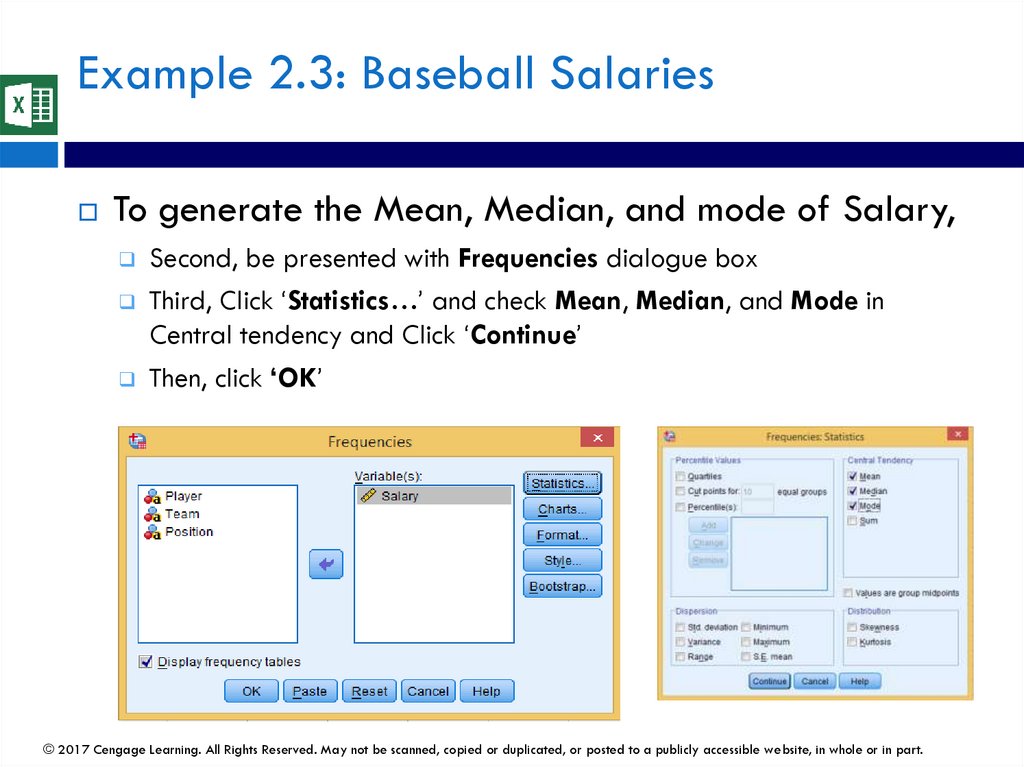
Example 2.3: Baseball SalariesTo generate the Mean, Median, and mode of Salary,
Second, be presented with Frequencies dialogue box
Third, Click ‘Statistics…’ and check Mean, Median, and Mode in
Central tendency and Click ‘Continue’
Then, click ‘OK’
© 2017 Cengage Learning. All Rights Reserved. May not be scanned, copied or duplicated, or posted to a publicly accessible website, in whole or in part.
87.
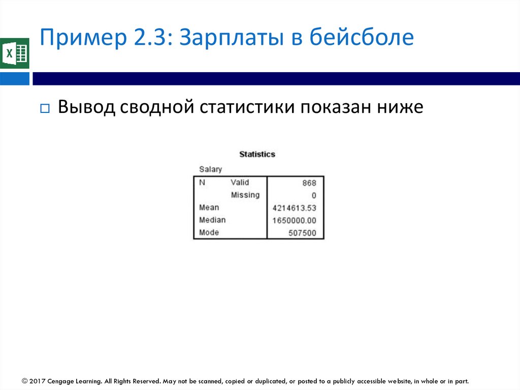
Пример 2.3: Зарплаты в бейсболеВывод сводной статистики показан ниже
© 2017 Cengage Learning. All Rights Reserved. May not be scanned, copied or duplicated, or posted to a publicly accessible website, in whole or in part.
88.
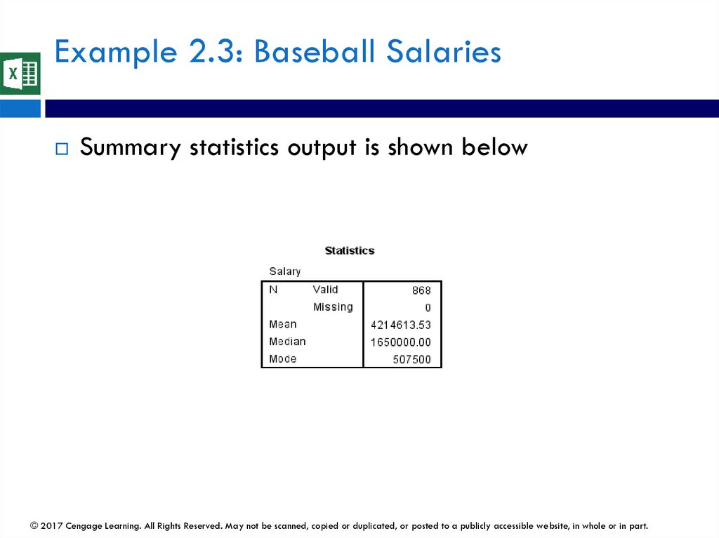
Example 2.3: Baseball SalariesSummary statistics output is shown below
© 2017 Cengage Learning. All Rights Reserved. May not be scanned, copied or duplicated, or posted to a publicly accessible website, in whole or in part.
89.
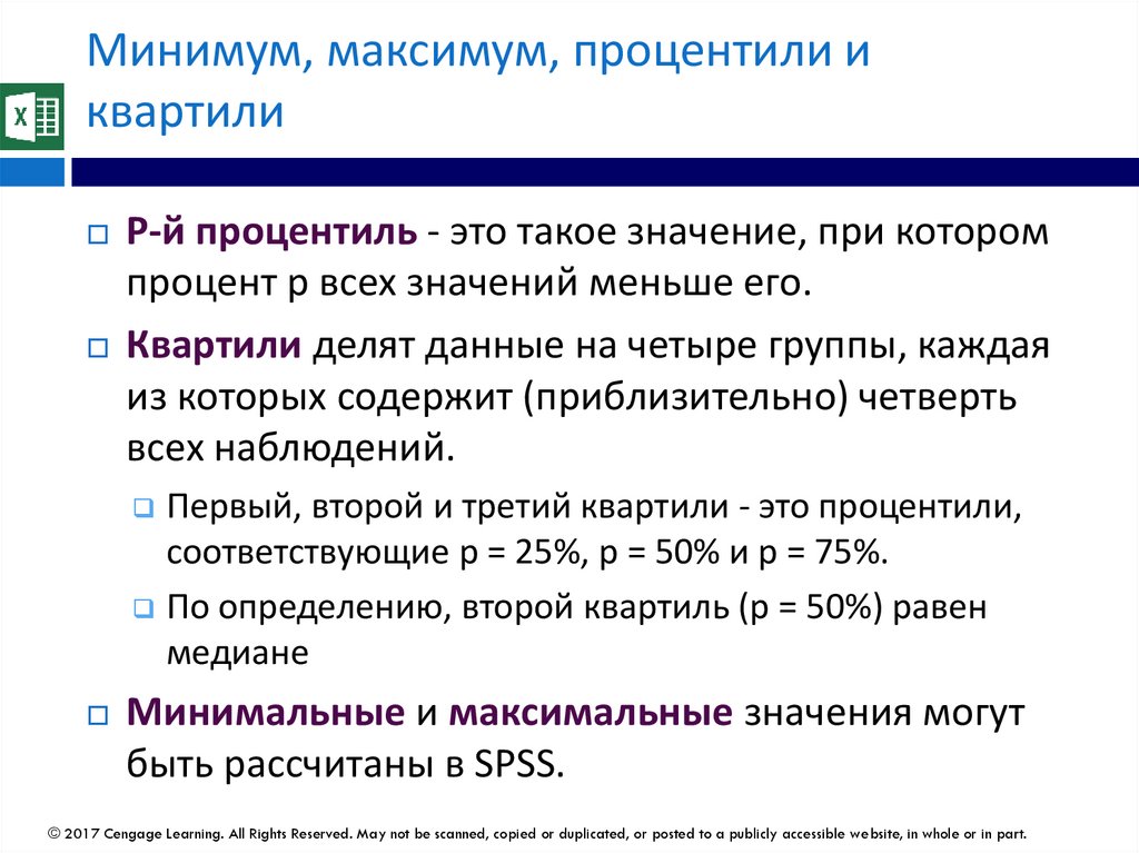
Минимум, максимум, процентили иквартили
P-й процентиль - это такое значение, при котором
процент p всех значений меньше его.
Квартили делят данные на четыре группы, каждая
из которых содержит (приблизительно) четверть
всех наблюдений.
Первый, второй и третий квартили - это процентили,
соответствующие p = 25%, p = 50% и p = 75%.
По определению, второй квартиль (p = 50%) равен
медиане
Минимальные и максимальные значения могут
быть рассчитаны в SPSS.
© 2017 Cengage Learning. All Rights Reserved. May not be scanned, copied or duplicated, or posted to a publicly accessible website, in whole or in part.
90.
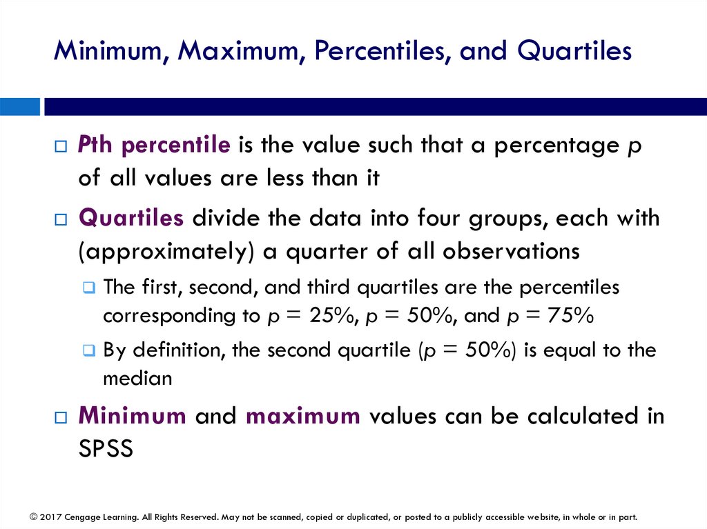
Minimum, Maximum, Percentiles, and QuartilesPth percentile is the value such that a percentage p
of all values are less than it
Quartiles divide the data into four groups, each with
(approximately) a quarter of all observations
The first, second, and third quartiles are the percentiles
corresponding to p = 25%, p = 50%, and p = 75%
By definition, the second quartile (p = 50%) is equal to the
median
Minimum and maximum values can be calculated in
SPSS
© 2017 Cengage Learning. All Rights Reserved. May not be scanned, copied or duplicated, or posted to a publicly accessible website, in whole or in part.
91.
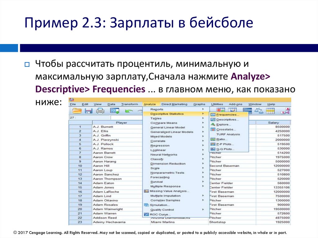
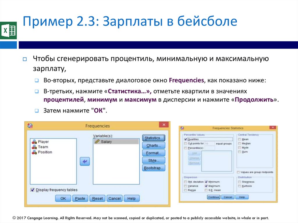
Пример 2.3: Зарплаты в бейсболеЧтобы рассчитать процентиль, минимальную и
максимальную зарплату,Сначала нажмите Analyze>
Descriptive> Frequencies ... в главном меню, как показано
ниже:
© 2017 Cengage Learning. All Rights Reserved. May not be scanned, copied or duplicated, or posted to a publicly accessible website, in whole or in part.
92.
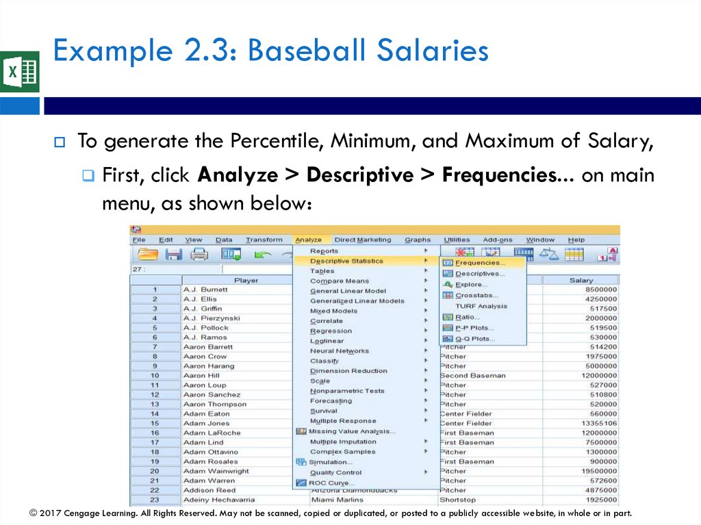
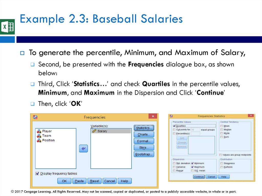
Example 2.3: Baseball SalariesTo generate the Percentile, Minimum, and Maximum of Salary,
First, click Analyze > Descriptive > Frequencies... on main
menu, as shown below:
© 2017 Cengage Learning. All Rights Reserved. May not be scanned, copied or duplicated, or posted to a publicly accessible website, in whole or in part.
93.
Пример 2.3: Зарплаты в бейсболеЧтобы сгенерировать процентиль, минимальную и максимальную
зарплату,
Во-вторых, представьте диалоговое окно Frequencies, как показано ниже:
В-третьих, нажмите «Статистика…», отметьте квартили в значениях
процентилей, минимум и максимум в дисперсии и нажмите «Продолжить».
Затем нажмите "ОК".
© 2017 Cengage Learning. All Rights Reserved. May not be scanned, copied or duplicated, or posted to a publicly accessible website, in whole or in part.
94.
Example 2.3: Baseball SalariesTo generate the percentile, Minimum, and Maximum of Salary,
Second, be presented with the Frequencies dialogue box, as shown
below:
Third, Click ‘Statistics…’ and check Quartiles in the percentile values,
Minimum, and Maximum in the Dispersion and Click ‘Continue’
Then, click ‘OK’
© 2017 Cengage Learning. All Rights Reserved. May not be scanned, copied or duplicated, or posted to a publicly accessible website, in whole or in part.
95.
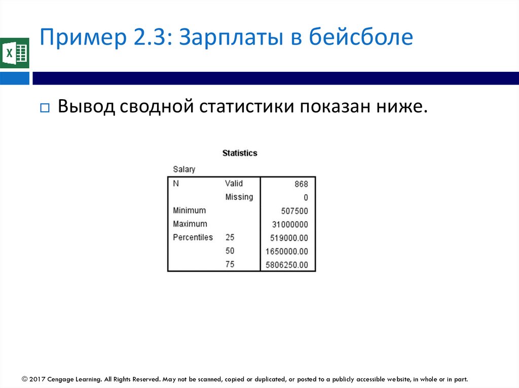
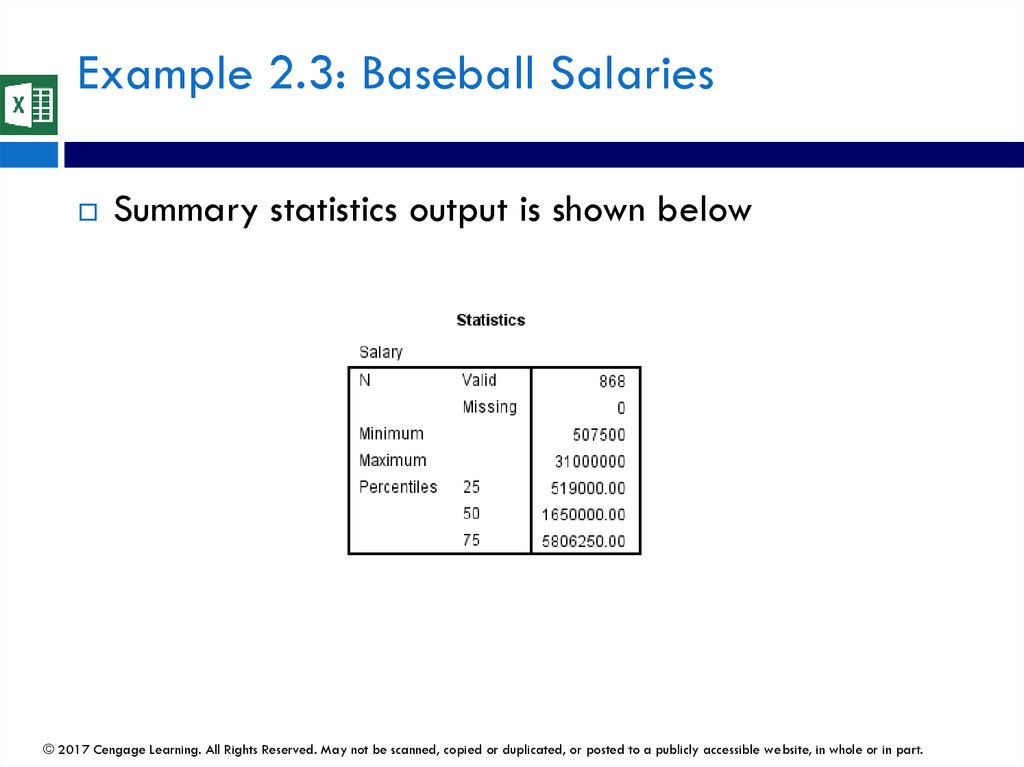
Пример 2.3: Зарплаты в бейсболеВывод сводной статистики показан ниже.
© 2017 Cengage Learning. All Rights Reserved. May not be scanned, copied or duplicated, or posted to a publicly accessible website, in whole or in part.
96.
Example 2.3: Baseball SalariesSummary statistics output is shown below
© 2017 Cengage Learning. All Rights Reserved. May not be scanned, copied or duplicated, or posted to a publicly accessible website, in whole or in part.
97.
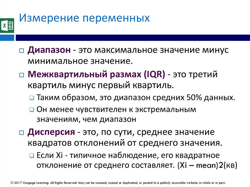
Измерение переменныхДиапазон - это максимальное значение минус
минимальное значение.
Межквартильный размах (IQR) - это третий
квартиль минус первый квартиль.
Таким образом, это диапазон средних 50% данных.
Он менее чувствителен к экстремальным
значениям, чем диапазон
Дисперсия - это, по сути, среднее значение
квадратов отклонений от среднего значения.
Если Xi - типичное наблюдение, его квадратное
отклонение от среднего составляет. (Xi – mean)2(кв)
© 2017 Cengage Learning. All Rights Reserved. May not be scanned, copied or duplicated, or posted to a publicly accessible website, in whole or in part.
98.
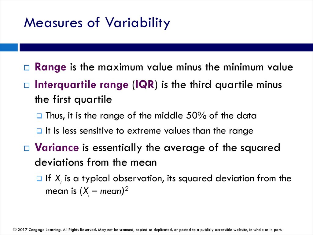
Measures of VariabilityRange is the maximum value minus the minimum value
Interquartile range (IQR) is the third quartile minus
the first quartile
Thus, it is the range of the middle 50% of the data
It is less sensitive to extreme values than the range
Variance is essentially the average of the squared
deviations from the mean
If Xi is a typical observation, its squared deviation from the
mean is (Xi – mean)2
© 2017 Cengage Learning. All Rights Reserved. May not be scanned, copied or duplicated, or posted to a publicly accessible website, in whole or in part.
99.
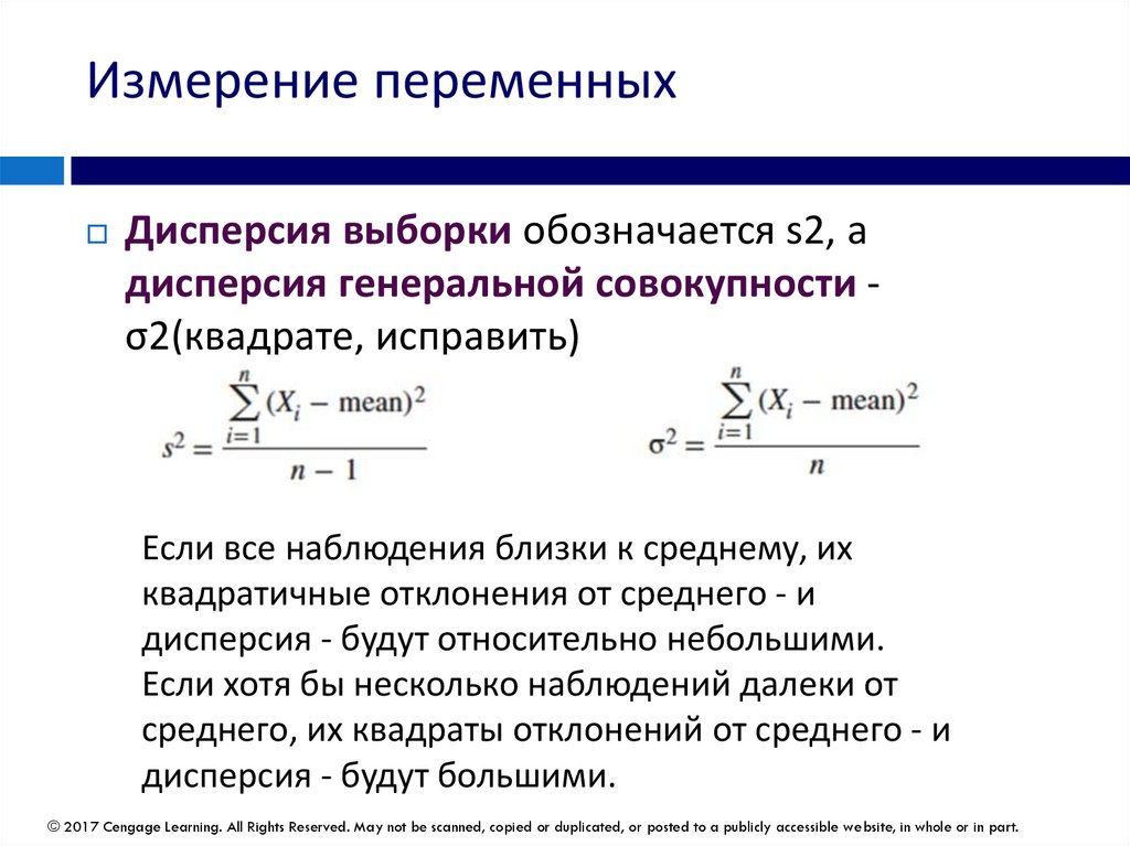
Измерение переменныхДисперсия выборки обозначается s2, а
дисперсия генеральной совокупности σ2(квадрате, исправить)
Если все наблюдения близки к среднему, их
квадратичные отклонения от среднего - и
дисперсия - будут относительно небольшими.
Если хотя бы несколько наблюдений далеки от
среднего, их квадраты отклонений от среднего - и
дисперсия - будут большими.
© 2017 Cengage Learning. All Rights Reserved. May not be scanned, copied or duplicated, or posted to a publicly accessible website, in whole or in part.
100.
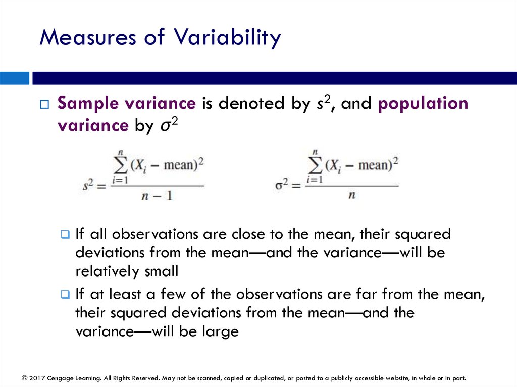
Measures of VariabilitySample variance is denoted by s2, and population
variance by σ2
If all observations are close to the mean, their squared
deviations from the mean—and the variance—will be
relatively small
If at least a few of the observations are far from the mean,
their squared deviations from the mean—and the
variance—will be large
© 2017 Cengage Learning. All Rights Reserved. May not be scanned, copied or duplicated, or posted to a publicly accessible website, in whole or in part.
101.
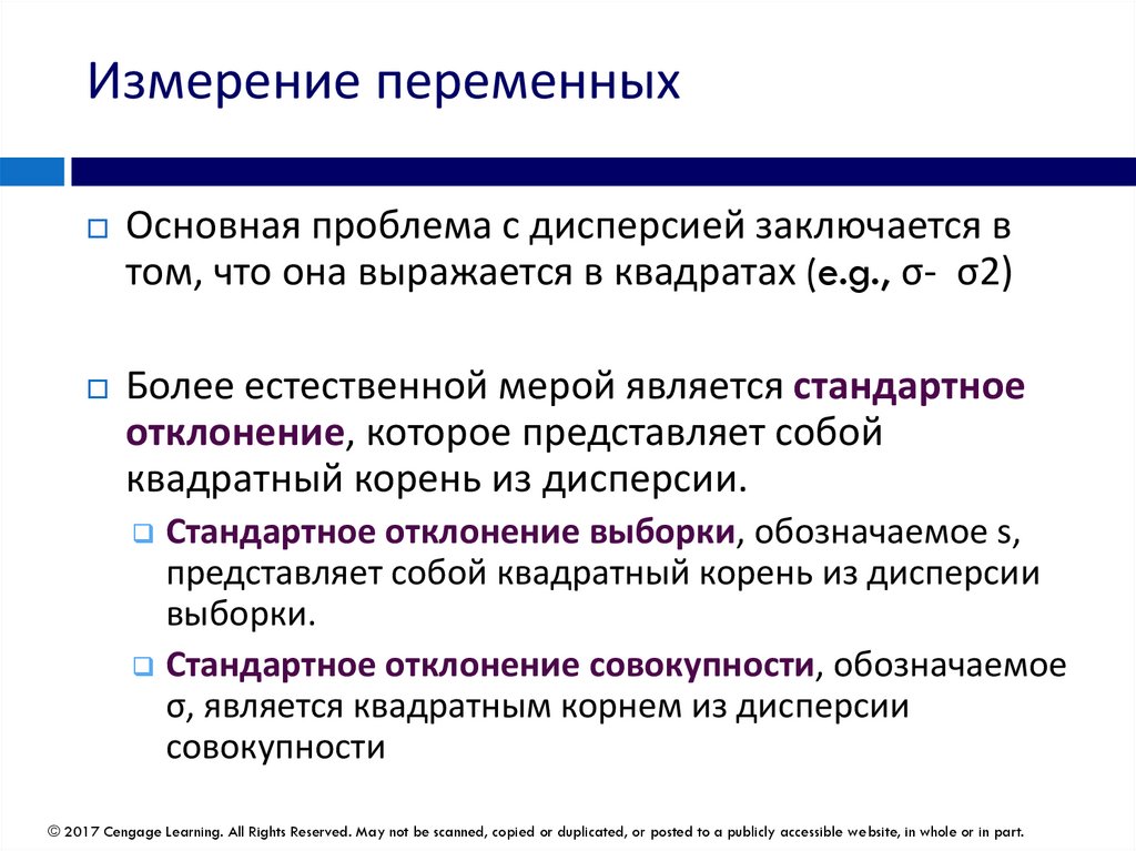
Измерение переменныхОсновная проблема с дисперсией заключается в
том, что она выражается в квадратах (e.g., σ- σ2)
Более естественной мерой является стандартное
отклонение, которое представляет собой
квадратный корень из дисперсии.
Стандартное отклонение выборки, обозначаемое s,
представляет собой квадратный корень из дисперсии
выборки.
Стандартное отклонение совокупности, обозначаемое
σ, является квадратным корнем из дисперсии
совокупности
© 2017 Cengage Learning. All Rights Reserved. May not be scanned, copied or duplicated, or posted to a publicly accessible website, in whole or in part.
102.
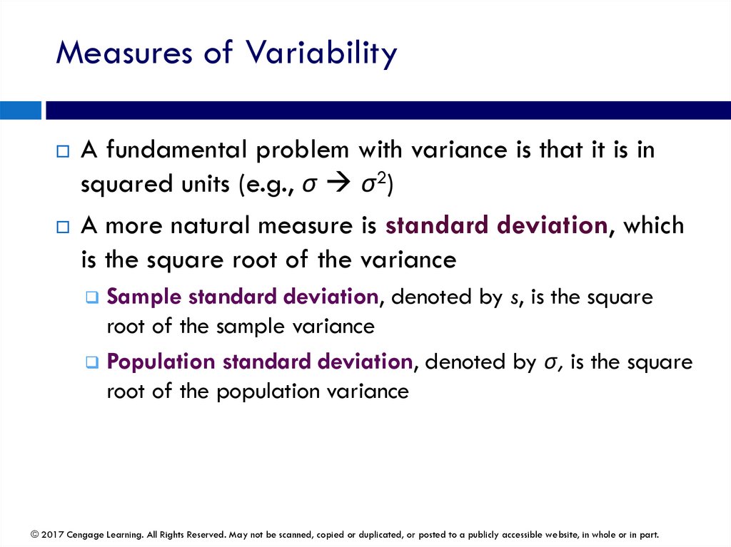
Measures of VariabilityA fundamental problem with variance is that it is in
squared units (e.g., σ σ2)
A more natural measure is standard deviation, which
is the square root of the variance
Sample standard deviation, denoted by s, is the square
root of the sample variance
Population standard deviation, denoted by σ, is the square
root of the population variance
© 2017 Cengage Learning. All Rights Reserved. May not be scanned, copied or duplicated, or posted to a publicly accessible website, in whole or in part.
103.
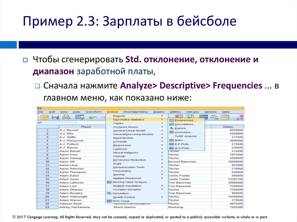
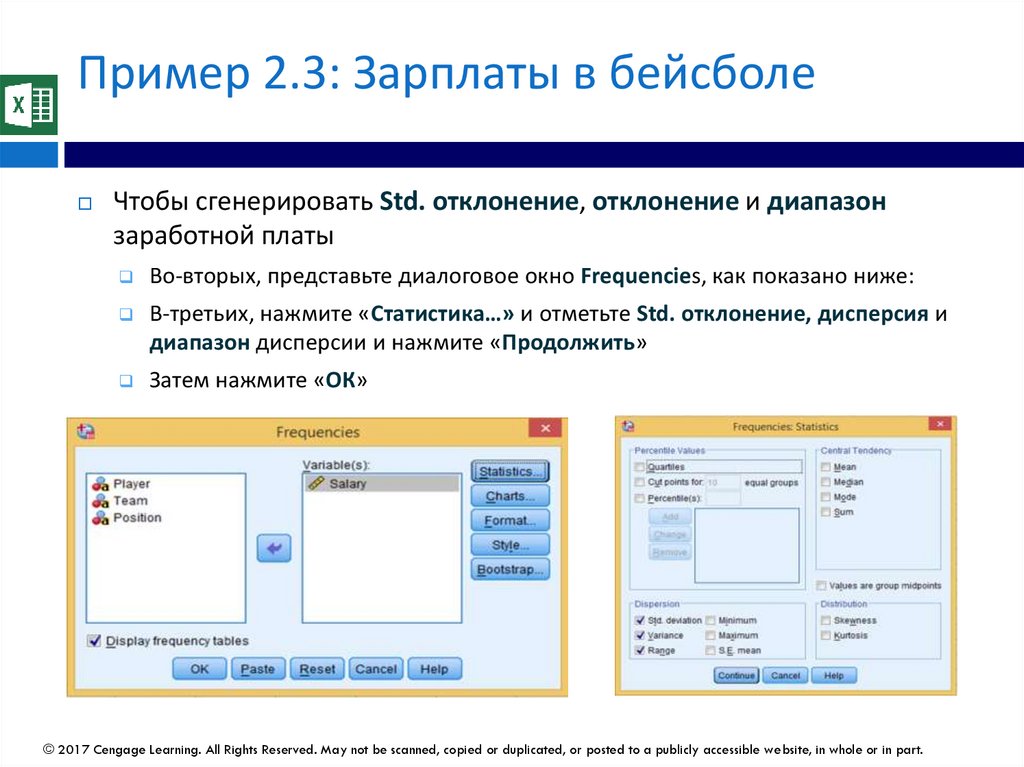
Пример 2.3: Зарплаты в бейсболеЧтобы сгенерировать Std. отклонение, отклонение и
диапазон заработной платы,
Сначала нажмите Analyze> Descriptive> Frequencies ... в
главном меню, как показано ниже:
© 2017 Cengage Learning. All Rights Reserved. May not be scanned, copied or duplicated, or posted to a publicly accessible website, in whole or in part.
104.
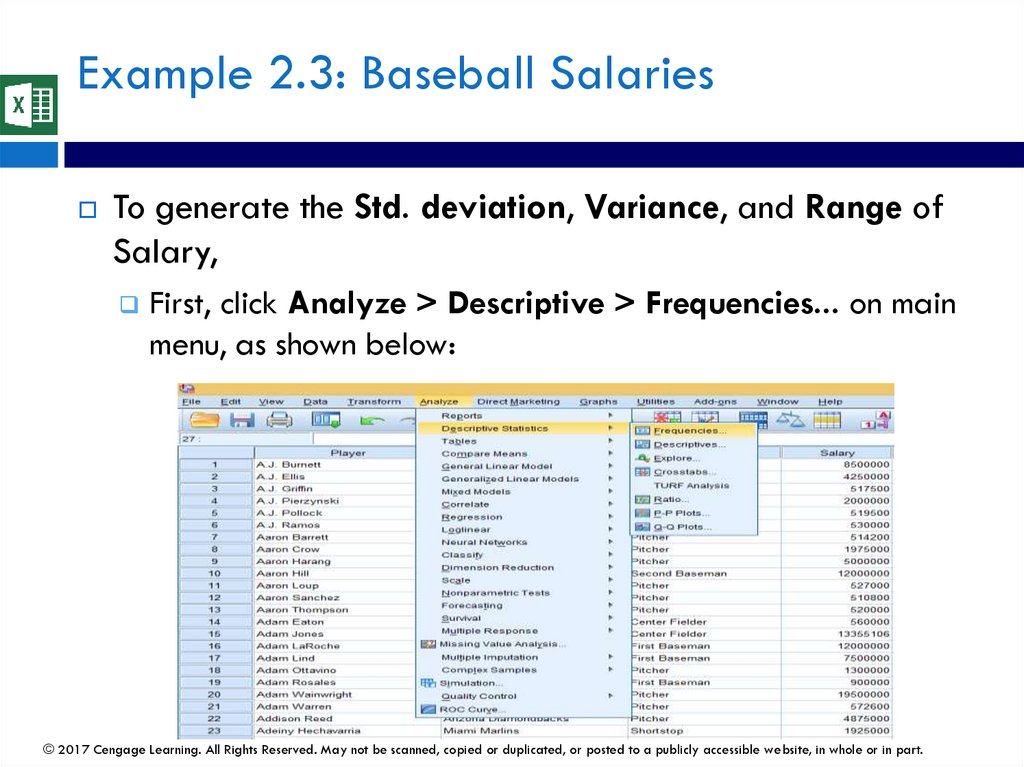
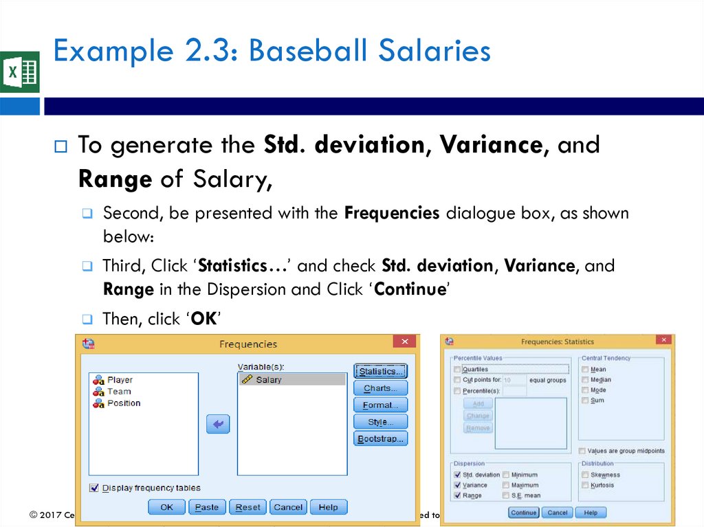
Example 2.3: Baseball SalariesTo generate the Std. deviation, Variance, and Range of
Salary,
First, click Analyze > Descriptive > Frequencies... on main
menu, as shown below:
© 2017 Cengage Learning. All Rights Reserved. May not be scanned, copied or duplicated, or posted to a publicly accessible website, in whole or in part.
105.
Пример 2.3: Зарплаты в бейсболеЧтобы сгенерировать Std. отклонение, отклонение и диапазон
заработной платы
Во-вторых, представьте диалоговое окно Frequencies, как показано ниже:
В-третьих, нажмите «Статистика…» и отметьте Std. отклонение, дисперсия и
диапазон дисперсии и нажмите «Продолжить»
Затем нажмите «ОК»
© 2017 Cengage Learning. All Rights Reserved. May not be scanned, copied or duplicated, or posted to a publicly accessible website, in whole or in part.
106.
Example 2.3: Baseball SalariesTo generate the Std. deviation, Variance, and
Range of Salary,
Second, be presented with the Frequencies dialogue box, as shown
below:
Third, Click ‘Statistics…’ and check Std. deviation, Variance, and
Range in the Dispersion and Click ‘Continue’
Then, click ‘OK’
© 2017 Cengage Learning. All Rights Reserved. May not be scanned, copied or duplicated, or posted to a publicly accessible website, in whole or in part.
107.
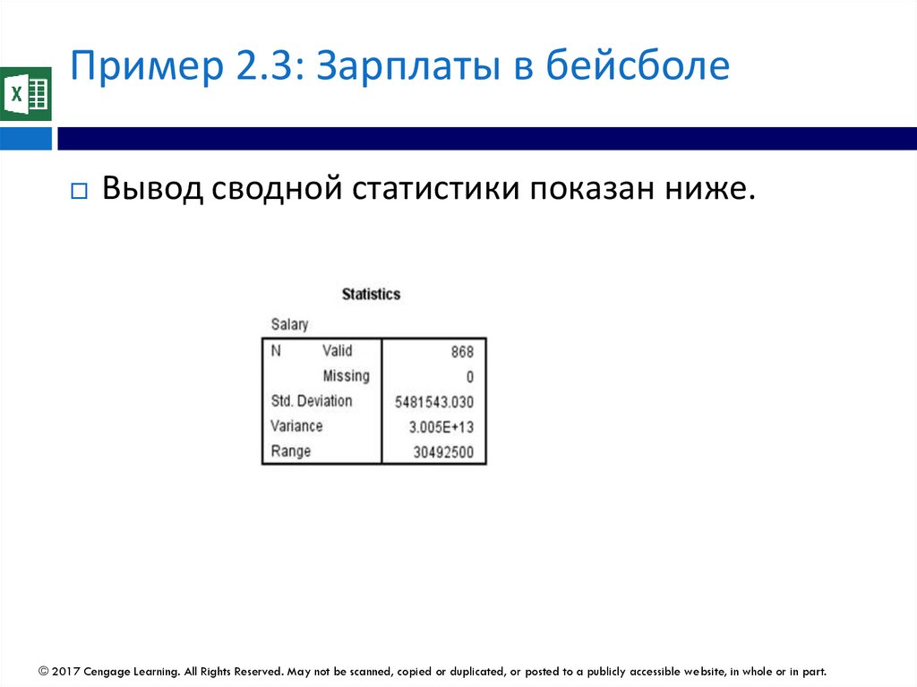
Пример 2.3: Зарплаты в бейсболеВывод сводной статистики показан ниже.
© 2017 Cengage Learning. All Rights Reserved. May not be scanned, copied or duplicated, or posted to a publicly accessible website, in whole or in part.
108.
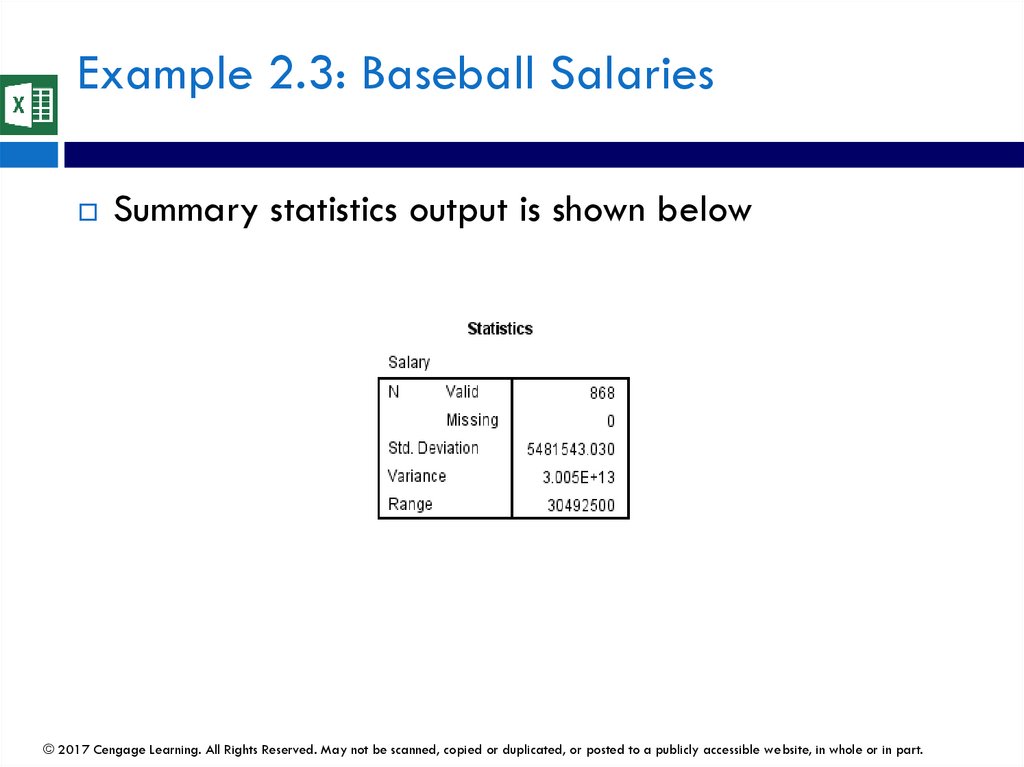
Example 2.3: Baseball SalariesSummary statistics output is shown below
© 2017 Cengage Learning. All Rights Reserved. May not be scanned, copied or duplicated, or posted to a publicly accessible website, in whole or in part.
109.
Эмпирические правила интерпретациистандартного отклонения
Интерпретацию стандартного отклонения можно
сформулировать как три эмпирических правила.
«Эмпирические» означает, что они основаны на обычно
наблюдаемых данных, а не на теоретических и
математических аргументах.
Если значения переменной имеют приблизительно
нормальное распределение (симметричное и
колоколообразное), то выполняются следующие
правила:
Примерно 68% наблюдений находятся в пределах одного
стандартного отклонения от среднего.
Примерно 95% наблюдений находятся в пределах двух
стандартных отклонений от среднего значения.
Примерно 99,7% наблюдений находятся в пределах трех
стандартных отклонений от среднего
© 2017 Cengage Learning. All Rights Reserved. May not be scanned, copied or duplicated, or posted to a publicly accessible website, in whole or in part.
110.
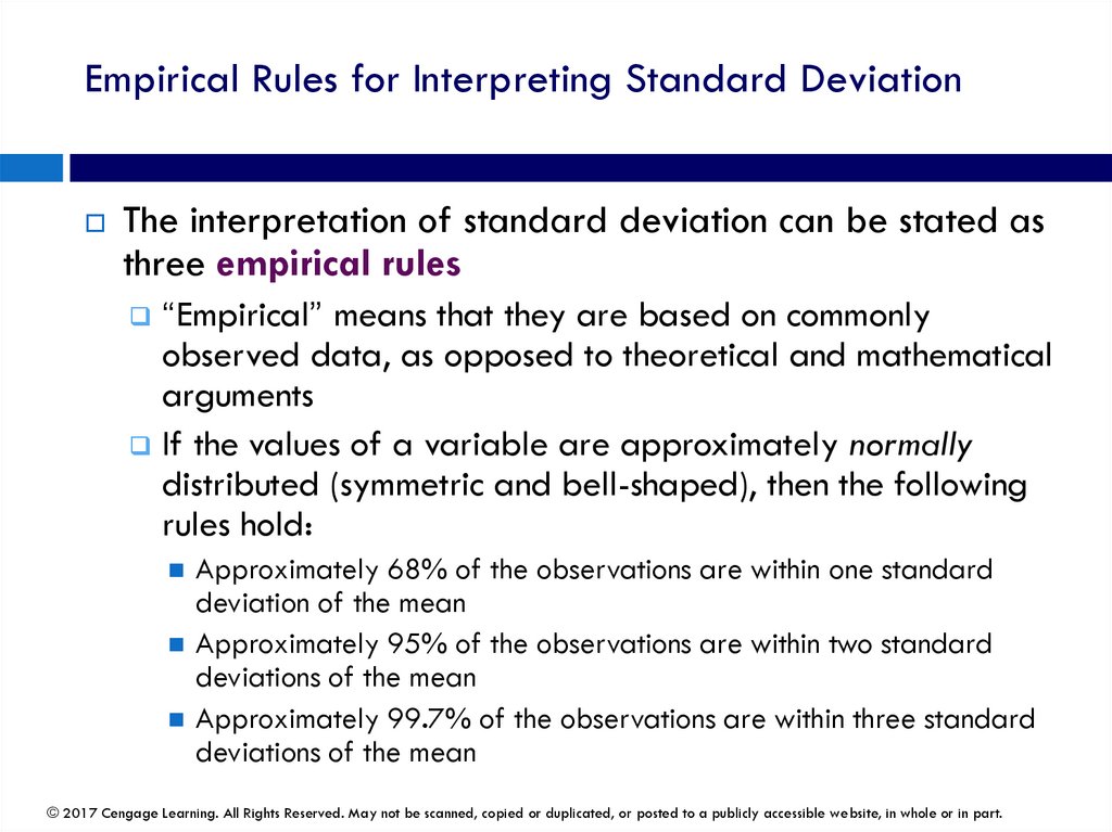
Empirical Rules for Interpreting Standard DeviationThe interpretation of standard deviation can be stated as
three empirical rules
“Empirical” means that they are based on commonly
observed data, as opposed to theoretical and mathematical
arguments
If the values of a variable are approximately normally
distributed (symmetric and bell-shaped), then the following
rules hold:
Approximately 68% of the observations are within one standard
deviation of the mean
Approximately 95% of the observations are within two standard
deviations of the mean
Approximately 99.7% of the observations are within three standard
deviations of the mean
© 2017 Cengage Learning. All Rights Reserved. May not be scanned, copied or duplicated, or posted to a publicly accessible website, in whole or in part.
111.
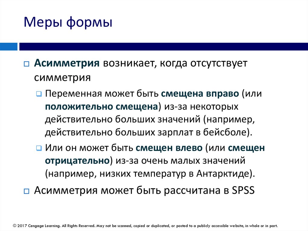
Меры формыАсимметрия возникает, когда отсутствует
симметрия
Переменная может быть смещена вправо (или
положительно смещена) из-за некоторых
действительно больших значений (например,
действительно больших зарплат в бейсболе).
Или он может быть смещен влево (или смещен
отрицательно) из-за очень малых значений
(например, низких температур в Антарктиде).
Асимметрия может быть рассчитана в SPSS
© 2017 Cengage Learning. All Rights Reserved. May not be scanned, copied or duplicated, or posted to a publicly accessible website, in whole or in part.
112.
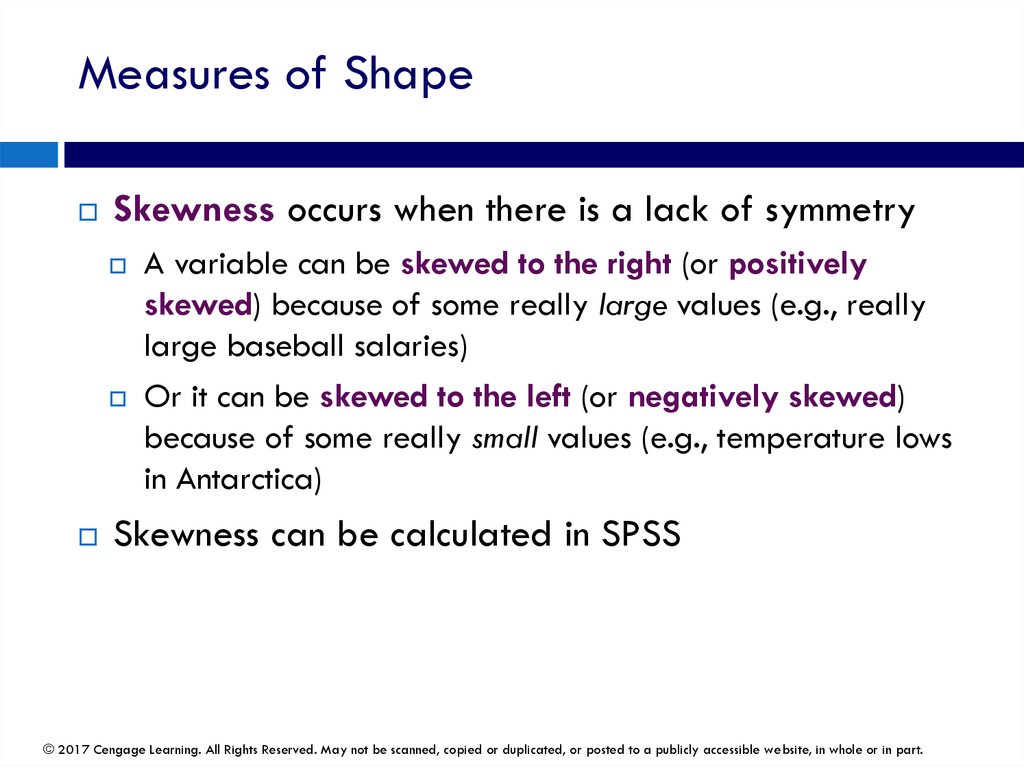
Measures of ShapeSkewness occurs when there is a lack of symmetry
A variable can be skewed to the right (or positively
skewed) because of some really large values (e.g., really
large baseball salaries)
Or it can be skewed to the left (or negatively skewed)
because of some really small values (e.g., temperature lows
in Antarctica)
Skewness can be calculated in SPSS
© 2017 Cengage Learning. All Rights Reserved. May not be scanned, copied or duplicated, or posted to a publicly accessible website, in whole or in part.
113.
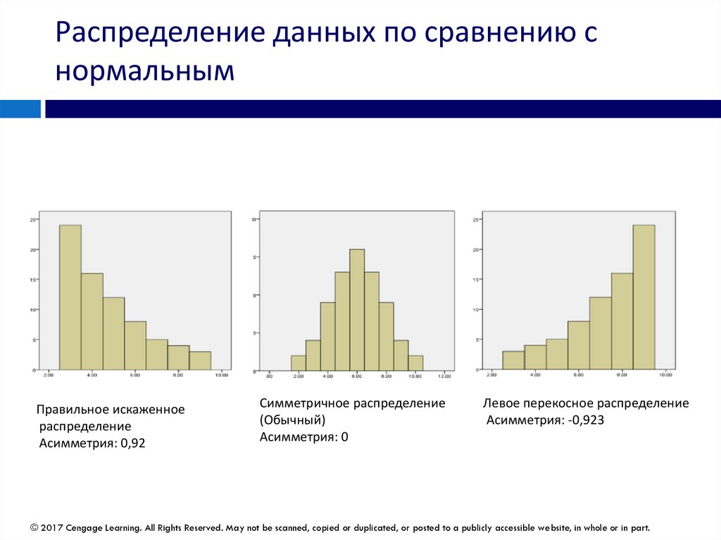
Распределение данных по сравнению снормальным
Правильное искаженное
распределение
Асимметрия: 0,92
Симметричное распределение
(Обычный)
Асимметрия: 0
Левое перекосное распределение
Асимметрия: -0,923
© 2017 Cengage Learning. All Rights Reserved. May not be scanned, copied or duplicated, or posted to a publicly accessible website, in whole or in part.
114.
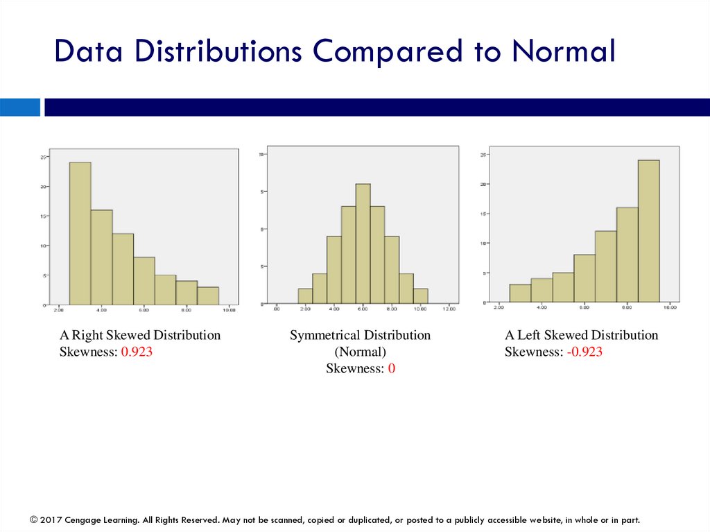
Data Distributions Compared to NormalA Right Skewed Distribution
Skewness: 0.923
Symmetrical Distribution
(Normal)
Skewness: 0
A Left Skewed Distribution
Skewness: -0.923
© 2017 Cengage Learning. All Rights Reserved. May not be scanned, copied or duplicated, or posted to a publicly accessible website, in whole or in part.
115.
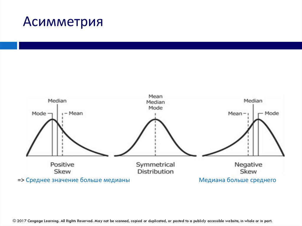
Асимметрия=> Среднее значение больше медианы
Медиана больше среднего
© 2017 Cengage Learning. All Rights Reserved. May not be scanned, copied or duplicated, or posted to a publicly accessible website, in whole or in part.
116.
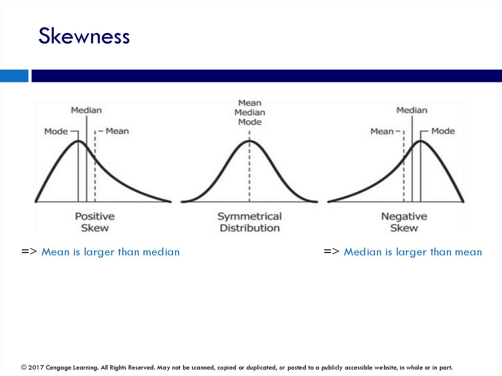
Skewness=> Mean is larger than median
=> Median is larger than mean
© 2017 Cengage Learning. All Rights Reserved. May not be scanned, copied or duplicated, or posted to a publicly accessible website, in whole or in part.
117.
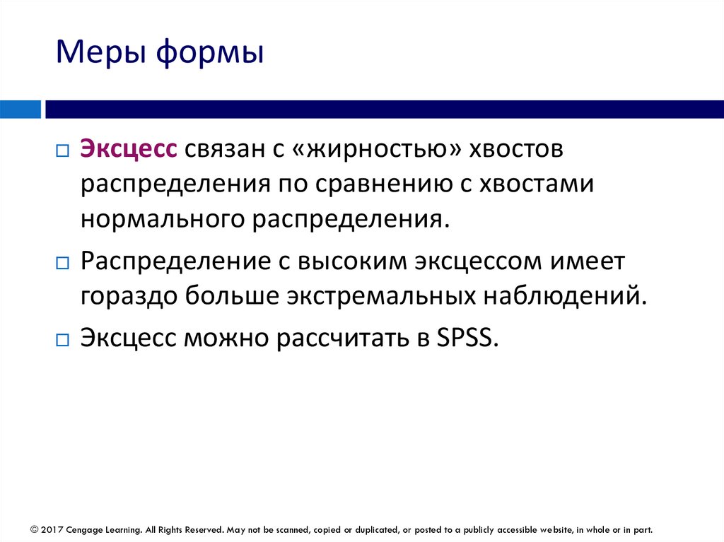
Меры формыЭксцесс связан с «жирностью» хвостов
распределения по сравнению с хвостами
нормального распределения.
Распределение с высоким эксцессом имеет
гораздо больше экстремальных наблюдений.
Эксцесс можно рассчитать в SPSS.
© 2017 Cengage Learning. All Rights Reserved. May not be scanned, copied or duplicated, or posted to a publicly accessible website, in whole or in part.
118.
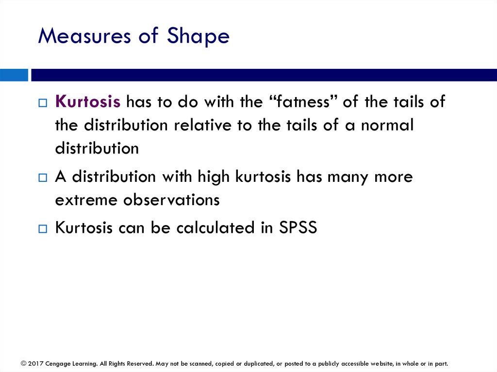
Measures of ShapeKurtosis has to do with the “fatness” of the tails of
the distribution relative to the tails of a normal
distribution
A distribution with high kurtosis has many more
extreme observations
Kurtosis can be calculated in SPSS
© 2017 Cengage Learning. All Rights Reserved. May not be scanned, copied or duplicated, or posted to a publicly accessible website, in whole or in part.
119.
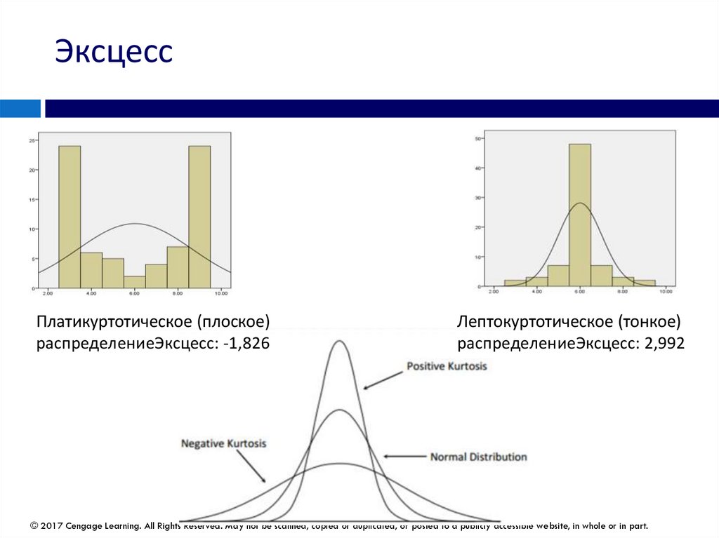
ЭксцессПлатикуртотическое (плоское)
распределениеЭксцесс: -1,826
Лептокуртотическое (тонкое)
распределениеЭксцесс: 2,992
© 2017 Cengage Learning. All Rights Reserved. May not be scanned, copied or duplicated, or posted to a publicly accessible website, in whole or in part.
120.
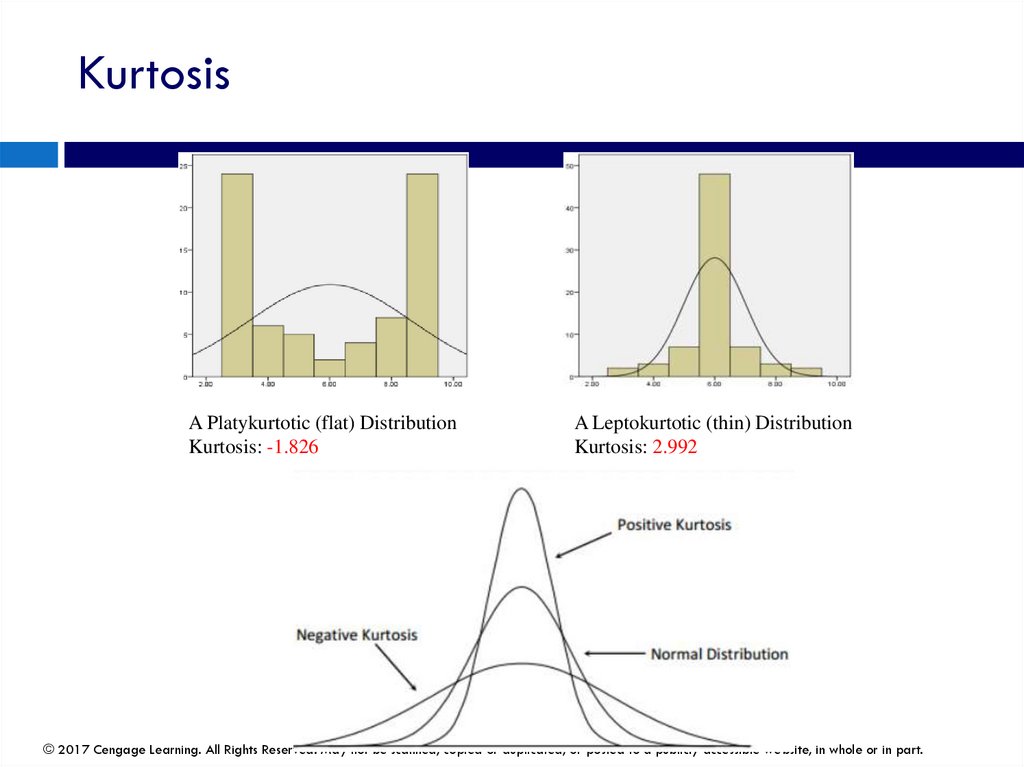
KurtosisA Platykurtotic (flat) Distribution
Kurtosis: -1.826
A Leptokurtotic (thin) Distribution
Kurtosis: 2.992
© 2017 Cengage Learning. All Rights Reserved. May not be scanned, copied or duplicated, or posted to a publicly accessible website, in whole or in part.
121.
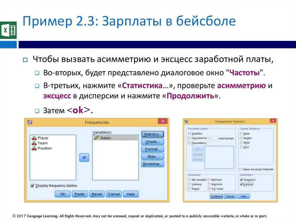
Пример 2.3: Зарплаты в бейсболеЧтобы вызвать асимметрию и эксцесс заработной платы,
Сначала нажмите Analyze> Descriptive> Frequencies ... в главном
меню, как показано ниже:
© 2017 Cengage Learning. All Rights Reserved. May not be scanned, copied or duplicated, or posted to a publicly accessible website, in whole or in part.
122.
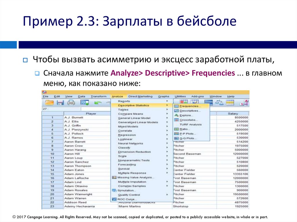
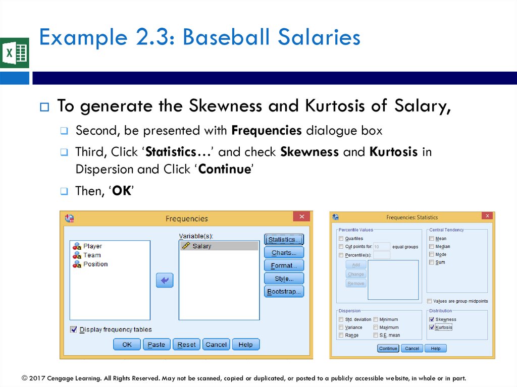
Example 2.3: Baseball SalariesTo generate the Skewness and Kurtosis of Salary,
First, click Analyze > Descriptive > Frequencies... On main
menu, as shown below:
© 2017 Cengage Learning. All Rights Reserved. May not be scanned, copied or duplicated, or posted to a publicly accessible website, in whole or in part.
123.
Пример 2.3: Зарплаты в бейсболеЧтобы вызвать асимметрию и эксцесс заработной платы,
Во-вторых, будет представлено диалоговое окно "Частоты".
В-третьих, нажмите «Статистика…», проверьте асимметрию и
эксцесс в дисперсии и нажмите «Продолжить».
Затем <
ok>.
© 2017 Cengage Learning. All Rights Reserved. May not be scanned, copied or duplicated, or posted to a publicly accessible website, in whole or in part.
124.
Example 2.3: Baseball SalariesTo generate the Skewness and Kurtosis of Salary,
Second, be presented with Frequencies dialogue box
Third, Click ‘Statistics…’ and check Skewness and Kurtosis in
Dispersion and Click ‘Continue’
Then, ‘OK’
© 2017 Cengage Learning. All Rights Reserved. May not be scanned, copied or duplicated, or posted to a publicly accessible website, in whole or in part.
125.
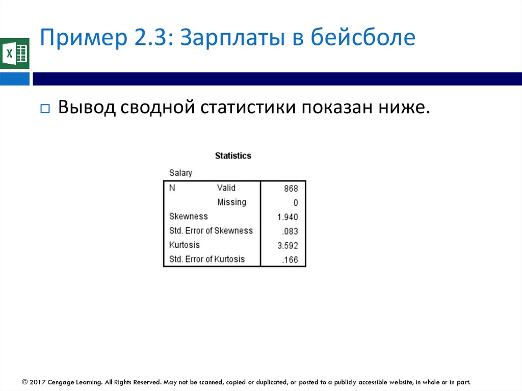
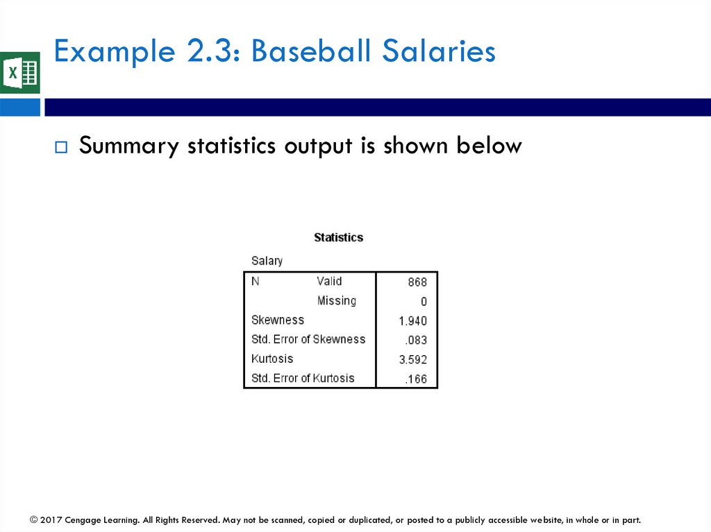
Пример 2.3: Зарплаты в бейсболеВывод сводной статистики показан ниже.
© 2017 Cengage Learning. All Rights Reserved. May not be scanned, copied or duplicated, or posted to a publicly accessible website, in whole or in part.
126.
Example 2.3: Baseball SalariesSummary statistics output is shown below
© 2017 Cengage Learning. All Rights Reserved. May not be scanned, copied or duplicated, or posted to a publicly accessible website, in whole or in part.
127.
2-4d графики для числовых переменныхСуществует множество графических способов
обозначения распределения числовой переменной.
Для поперечных переменных:
Гистограммы
Коробчатые диаграммы (коробчатые-усовидные
графики)
Для переменных временных рядов:
Графики временны
© 2017 Cengage Learning. All Rights Reserved. May not be scanned, copied or duplicated, or posted to a publicly accessible website, in whole or in part.
128.
2-4d Charts for Numerical VariablesThere are many graphical ways to indicate the
distribution of a numerical variable
For cross-sectional variables:
Histograms
Box plots (box-whisker plots)
For time series variables:
Time series graphs
© 2017 Cengage Learning. All Rights Reserved. May not be scanned, copied or duplicated, or posted to a publicly accessible website, in whole or in part.
129.
ГистограммыГистограмма - это наиболее распространенный тип
диаграммы для отображения распределения числовой
переменной.
Он основан на группировке переменной, то есть делении ее на
отдельные категории.
Это столбчатая диаграмма с подсчетами в различных
категориях.
Гистограмма отлично подходит для отображения формы
распределения - независимо от того, является ли
распределение симметричным или смещенным в одном
направлении.
© 2017 Cengage Learning. All Rights Reserved. May not be scanned, copied or duplicated, or posted to a publicly accessible website, in whole or in part.
130.
HistogramsHistogram is the most common type of chart for
showing the distribution of a numerical variable
It is based on binning the variable—that is, dividing it up
into discrete categories
It is a column chart of the counts in the various categories
Histogram is great for showing the shape of a
distribution—whether the distribution is symmetric or
skewed in one direction
© 2017 Cengage Learning. All Rights Reserved. May not be scanned, copied or duplicated, or posted to a publicly accessible website, in whole or in part.
131.
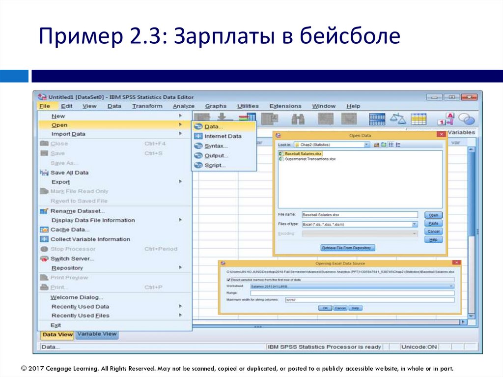
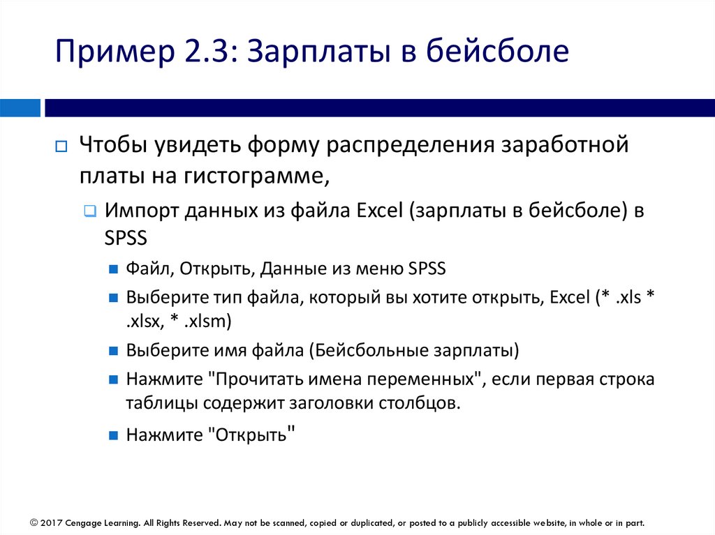
Пример 2.3: Зарплаты в бейсболеЧтобы увидеть форму распределения заработной
платы на гистограмме,
Импорт данных из файла Excel (зарплаты в бейсболе) в
SPSS
Файл, Открыть, Данные из меню SPSS
Выберите тип файла, который вы хотите открыть, Excel (* .xls *
.xlsx, * .xlsm)
Выберите имя файла (Бейсбольные зарплаты)
Нажмите "Прочитать имена переменных", если первая строка
таблицы содержит заголовки столбцов.
Нажмите "Открыть"
© 2017 Cengage Learning. All Rights Reserved. May not be scanned, copied or duplicated, or posted to a publicly accessible website, in whole or in part.
132.
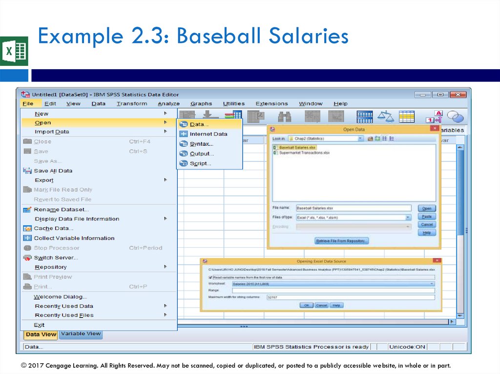
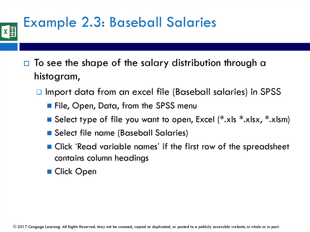
Example 2.3: Baseball SalariesTo see the shape of the salary distribution through a
histogram,
Import data from an excel file (Baseball salaries) in SPSS
File, Open, Data, from the SPSS menu
Select type of file you want to open, Excel (*.xls *.xlsx, *.xlsm)
Select file name (Baseball Salaries)
Click ‘Read variable names’ if the first row of the spreadsheet
contains column headings
Click Open
© 2017 Cengage Learning. All Rights Reserved. May not be scanned, copied or duplicated, or posted to a publicly accessible website, in whole or in part.
133.
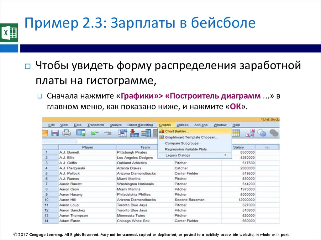
Пример 2.3: Зарплаты в бейсболеЧтобы увидеть форму распределения заработной
платы на гистограмме,
Сначала нажмите «Графики»> «Построитель диаграмм ...» в
главном меню, как показано ниже, и нажмите «ОК».
© 2017 Cengage Learning. All Rights Reserved. May not be scanned, copied or duplicated, or posted to a publicly accessible website, in whole or in part.
134.
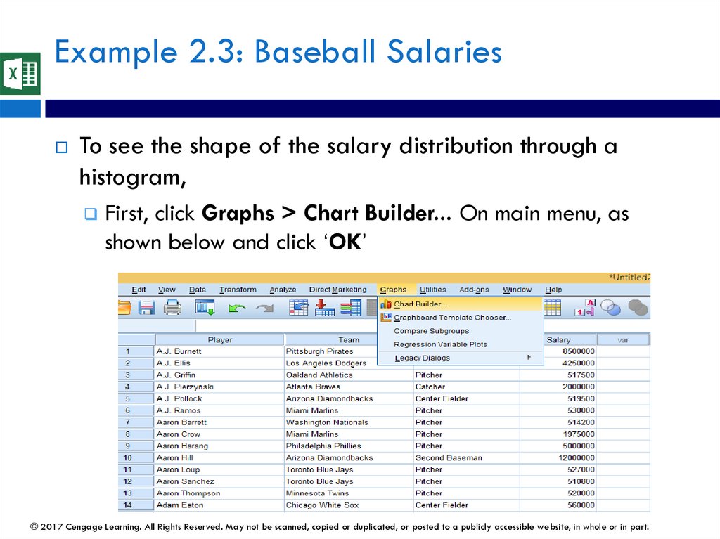
Example 2.3: Baseball SalariesTo see the shape of the salary distribution through a
histogram,
First, click Graphs > Chart Builder... On main menu, as
shown below and click ‘OK’
© 2017 Cengage Learning. All Rights Reserved. May not be scanned, copied or duplicated, or posted to a publicly accessible website, in whole or in part.
135.
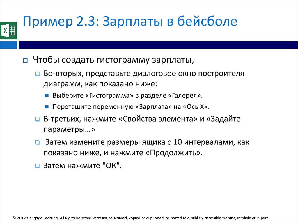
Пример 2.3: Зарплаты в бейсболеЧтобы создать гистограмму зарплаты,
Во-вторых, представьте диалоговое окно построителя
диаграмм, как показано ниже:
Выберите «Гистограмма» в разделе «Галерея».
Перетащите переменную «Зарплата» на «Ось X».
В-третьих, нажмите «Свойства элемента» и «Задайте
параметры…»
Затем измените размеры ящика с 10 интервалами, как
показано ниже, и нажмите «Продолжить».
Затем нажмите "ОК".
© 2017 Cengage Learning. All Rights Reserved. May not be scanned, copied or duplicated, or posted to a publicly accessible website, in whole or in part.
136.
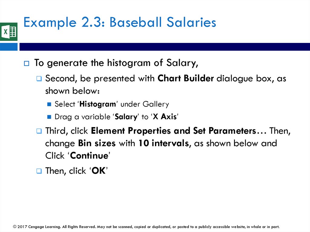
Example 2.3: Baseball SalariesTo generate the histogram of Salary,
Second, be presented with Chart Builder dialogue box, as
shown below:
Select ‘Histogram’ under Gallery
Drag a variable ‘Salary’ to ‘X Axis’
Third, click Element Properties and Set Parameters… Then,
change Bin sizes with 10 intervals, as shown below and
Click ‘Continue’
Then, click ‘OK’
© 2017 Cengage Learning. All Rights Reserved. May not be scanned, copied or duplicated, or posted to a publicly accessible website, in whole or in part.
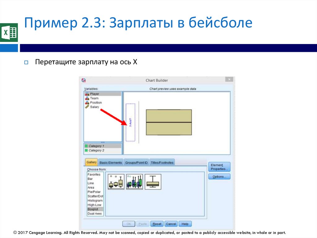
137.
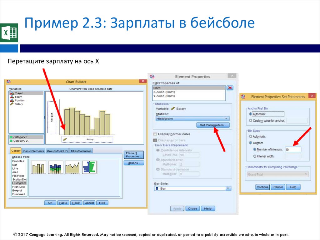
Пример 2.3: Зарплаты в бейсболеПеретащите зарплату на ось X
© 2017 Cengage Learning. All Rights Reserved. May not be scanned, copied or duplicated, or posted to a publicly accessible website, in whole or in part.
138.
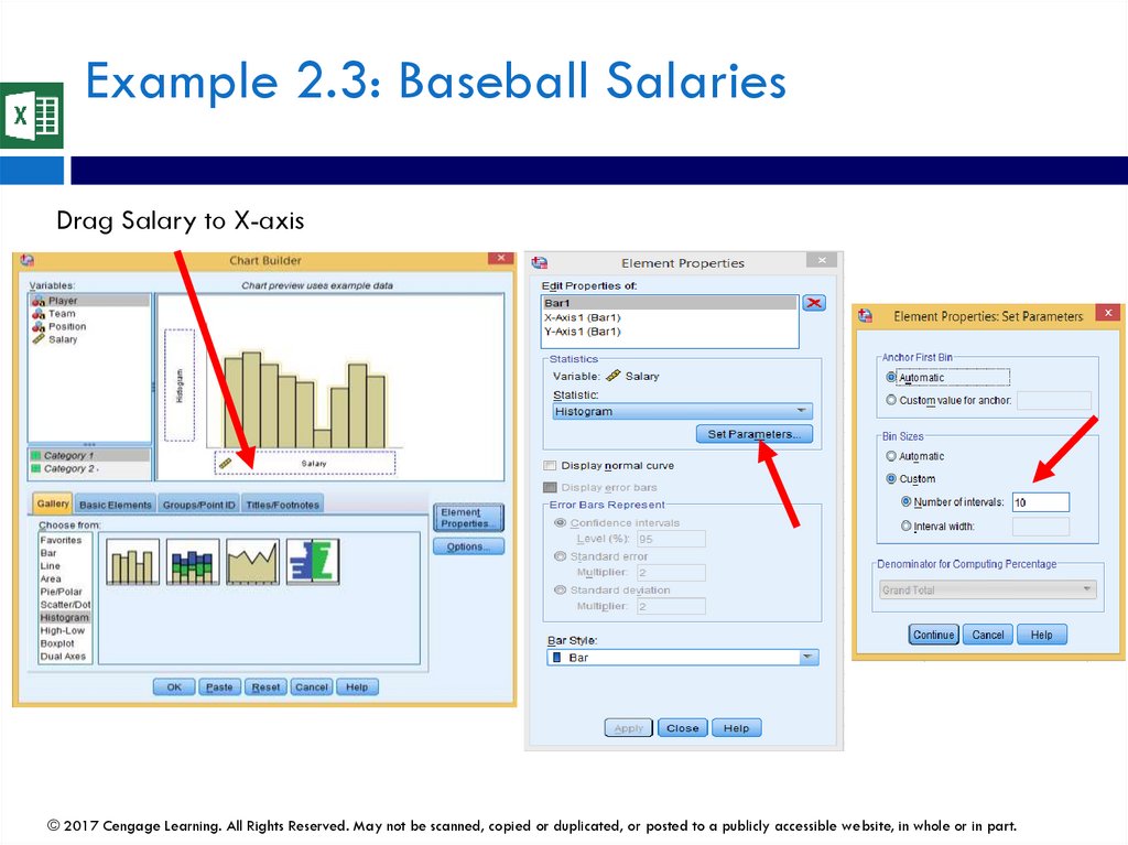
Example 2.3: Baseball SalariesDrag Salary to X-axis
© 2017 Cengage Learning. All Rights Reserved. May not be scanned, copied or duplicated, or posted to a publicly accessible website, in whole or in part.
139.
Пример 2.3: Зарплаты в бейсболеГистограмма зарплаты представлена ниже.
© 2017 Cengage Learning. All Rights Reserved. May not be scanned, copied or duplicated, or posted to a publicly accessible website, in whole or in part.
140.
Example 2.3: Baseball SalariesHistogram of Salary is shown below
© 2017 Cengage Learning. All Rights Reserved. May not be scanned, copied or duplicated, or posted to a publicly accessible website, in whole or in part.
141.
Коробчатые графики (Box Plots)Ящичковая диаграмма (или диаграмма ящика-
уса) - это альтернативный тип диаграммы для
отображения распределения переменной.
Параллельные ящичные диаграммы очень
полезны для сравнения распределений.
Ящичные диаграммы и гистограммы являются
дополнительными способами отображения
распределения числовой переменной.
Как и гистограммы, ящичные диаграммы
представляют собой диаграммы «общей картины».
© 2017 Cengage Learning. All Rights Reserved. May not be scanned, copied or duplicated, or posted to a publicly accessible website, in whole or in part.
142.
Box PlotsBox plot (or box-whisker plot) is an alternative type
of chart for showing the distribution of a variable
Side-by-side box plots are very useful for comparing
distributions
Box plots and histograms are complementary ways of
displaying the distribution of a numerical variable
As with histograms, box plots are “big picture” charts
© 2017 Cengage Learning. All Rights Reserved. May not be scanned, copied or duplicated, or posted to a publicly accessible website, in whole or in part.
143.
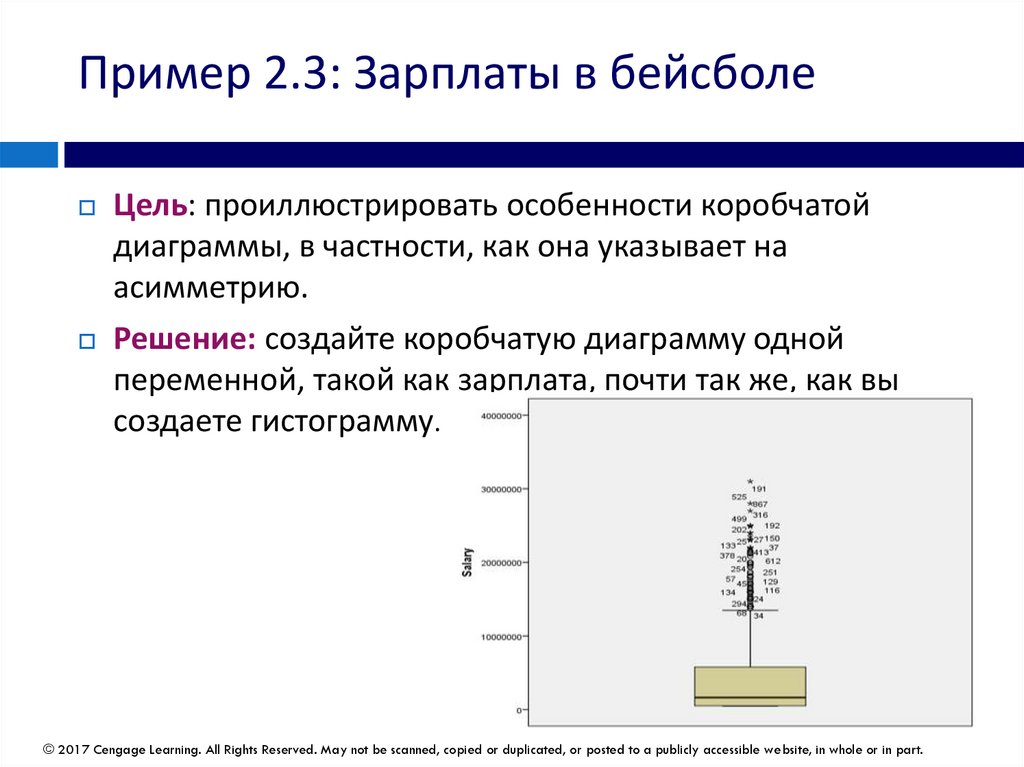
Пример 2.3: Зарплаты в бейсболеЦель: проиллюстрировать особенности коробчатой
диаграммы, в частности, как она указывает на
асимметрию.
Решение: создайте коробчатую диаграмму одной
переменной, такой как зарплата, почти так же, как вы
создаете гистограмму.
© 2017 Cengage Learning. All Rights Reserved. May not be scanned, copied or duplicated, or posted to a publicly accessible website, in whole or in part.
144.
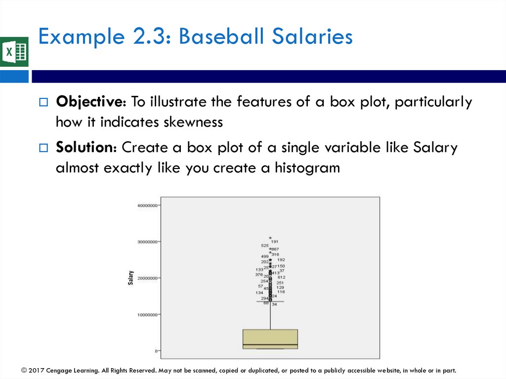
Example 2.3: Baseball SalariesObjective: To illustrate the features of a box plot, particularly
how it indicates skewness
Solution: Create a box plot of a single variable like Salary
almost exactly like you create a histogram
© 2017 Cengage Learning. All Rights Reserved. May not be scanned, copied or duplicated, or posted to a publicly accessible website, in whole or in part.
145.
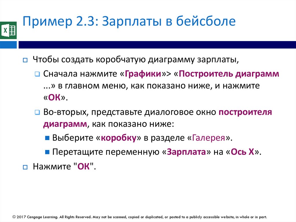
Пример 2.3: Зарплаты в бейсболеЧтобы создать коробчатую диаграмму зарплаты,
Сначала нажмите «Графики»> «Построитель диаграмм
...» в главном меню, как показано ниже, и нажмите
«ОК».
Во-вторых, представьте диалоговое окно построителя
диаграмм, как показано ниже:
Выберите «коробку» в разделе «Галерея».
Перетащите переменную «Зарплата» на «Ось X».
Нажмите "ОК".
© 2017 Cengage Learning. All Rights Reserved. May not be scanned, copied or duplicated, or posted to a publicly accessible website, in whole or in part.
146.
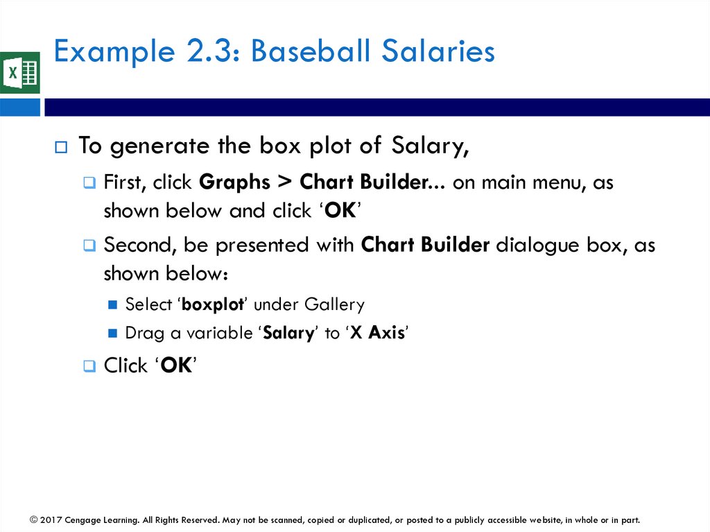
Example 2.3: Baseball SalariesTo generate the box plot of Salary,
First, click Graphs > Chart Builder... on main menu, as
shown below and click ‘OK’
Second, be presented with Chart Builder dialogue box, as
shown below:
Select ‘boxplot’ under Gallery
Drag a variable ‘Salary’ to ‘X Axis’
Click ‘OK’
© 2017 Cengage Learning. All Rights Reserved. May not be scanned, copied or duplicated, or posted to a publicly accessible website, in whole or in part.
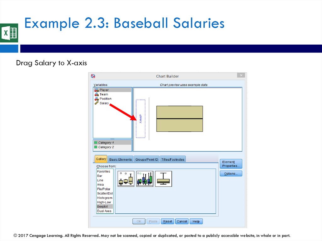
147.
Пример 2.3: Зарплаты в бейсболеПеретащите зарплату на ось X
© 2017 Cengage Learning. All Rights Reserved. May not be scanned, copied or duplicated, or posted to a publicly accessible website, in whole or in part.
148.
Example 2.3: Baseball SalariesDrag Salary to X-axis
© 2017 Cengage Learning. All Rights Reserved. May not be scanned, copied or duplicated, or posted to a publicly accessible website, in whole or in part.
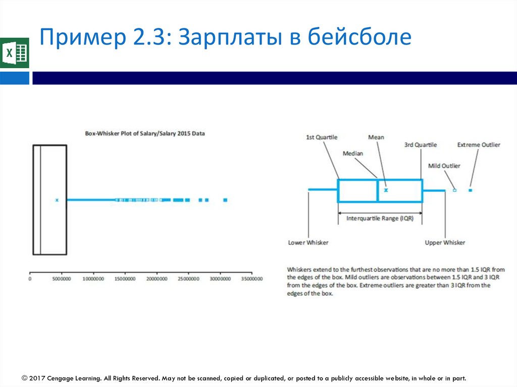
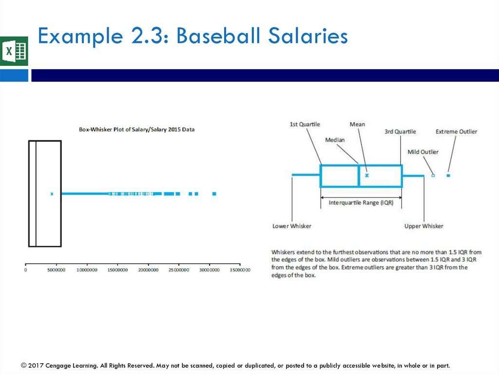
149.
Пример 2.3: Зарплаты в бейсболе© 2017 Cengage Learning. All Rights Reserved. May not be scanned, copied or duplicated, or posted to a publicly accessible website, in whole or in part.
150.
Example 2.3: Baseball Salaries© 2017 Cengage Learning. All Rights Reserved. May not be scanned, copied or duplicated, or posted to a publicly accessible website, in whole or in part.
151.
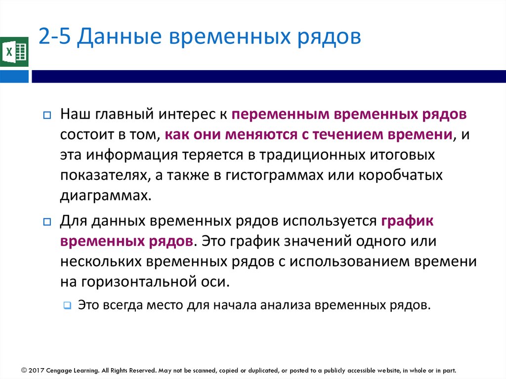
2-5 Данные временных рядовНаш главный интерес к переменным временных рядов
состоит в том, как они меняются с течением времени, и
эта информация теряется в традиционных итоговых
показателях, а также в гистограммах или коробчатых
диаграммах.
Для данных временных рядов используется график
временных рядов. Это график значений одного или
нескольких временных рядов с использованием времени
на горизонтальной оси.
Это всегда место для начала анализа временных рядов.
© 2017 Cengage Learning. All Rights Reserved. May not be scanned, copied or duplicated, or posted to a publicly accessible website, in whole or in part.
152.
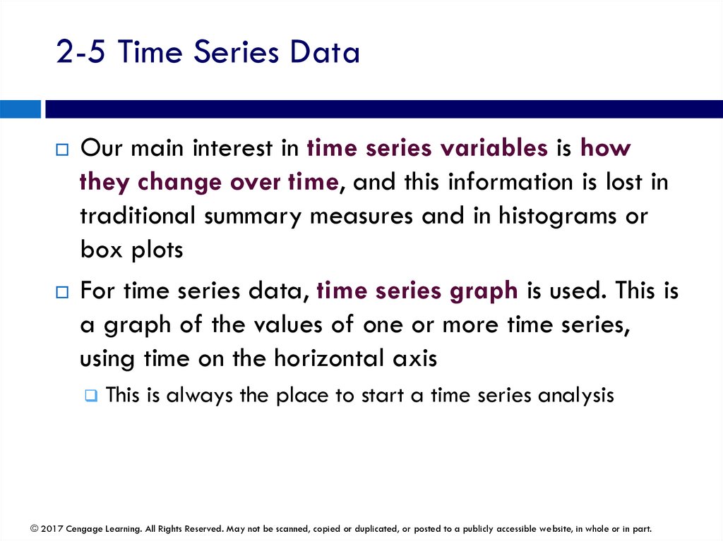
2-5 Time Series DataOur main interest in time series variables is how
they change over time, and this information is lost in
traditional summary measures and in histograms or
box plots
For time series data, time series graph is used. This is
a graph of the values of one or more time series,
using time on the horizontal axis
This is always the place to start a time series analysis
© 2017 Cengage Learning. All Rights Reserved. May not be scanned, copied or duplicated, or posted to a publicly accessible website, in whole or in part.
153.
Пример 2.4: Преступность в США© 2017 Cengage Learning. All Rights Reserved. May not be scanned, copied or duplicated, or posted to a publicly accessible website, in whole or in part.
154.
Example 2.4: Crime in United States© 2017 Cengage Learning. All Rights Reserved. May not be scanned, copied or duplicated, or posted to a publicly accessible website, in whole or in part.
155.
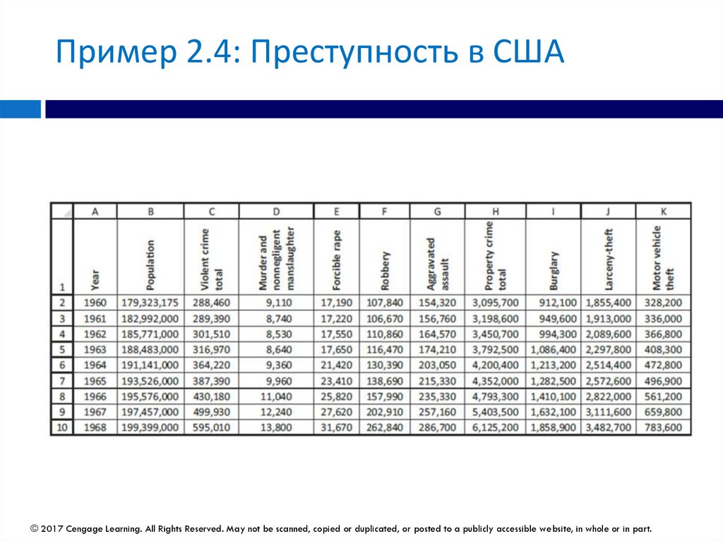
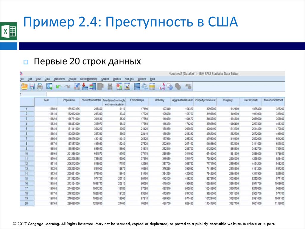
Пример 2.4: Преступность в СШАПервые 20 строк данных
© 2017 Cengage Learning. All Rights Reserved. May not be scanned, copied or duplicated, or posted to a publicly accessible website, in whole or in part.
156.
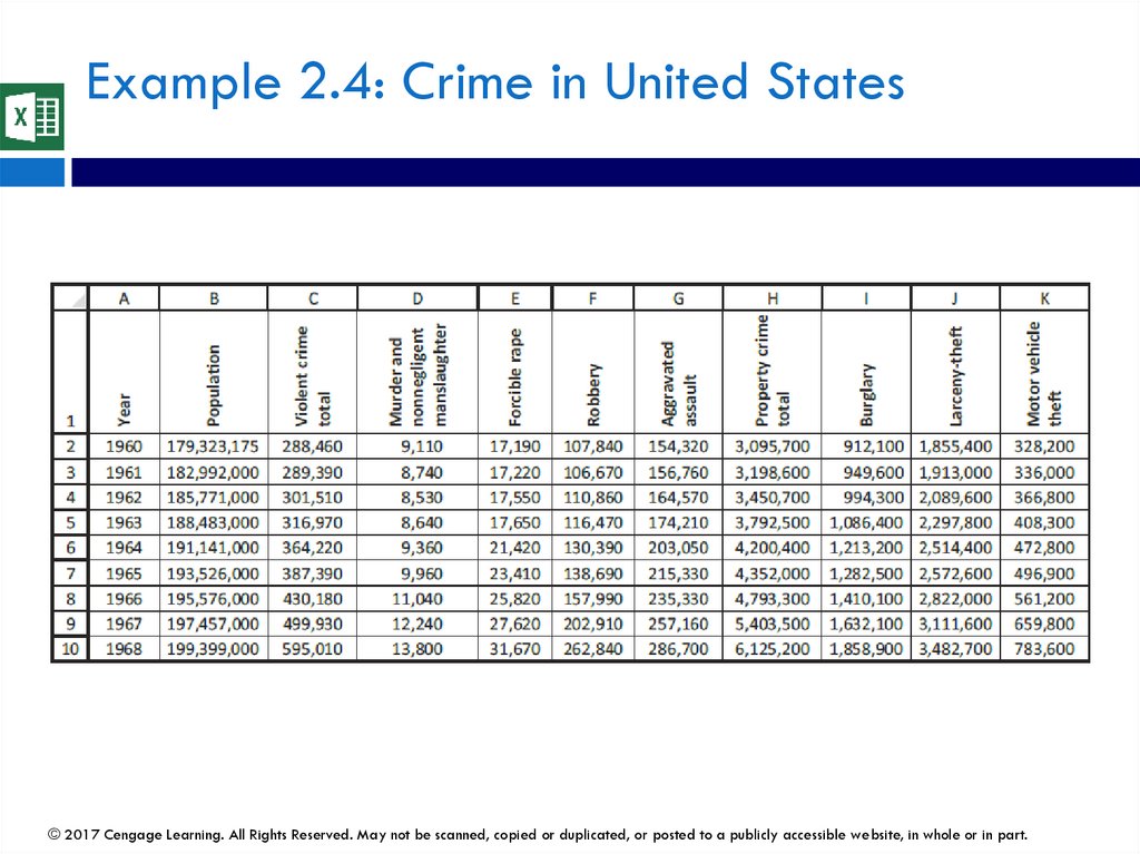
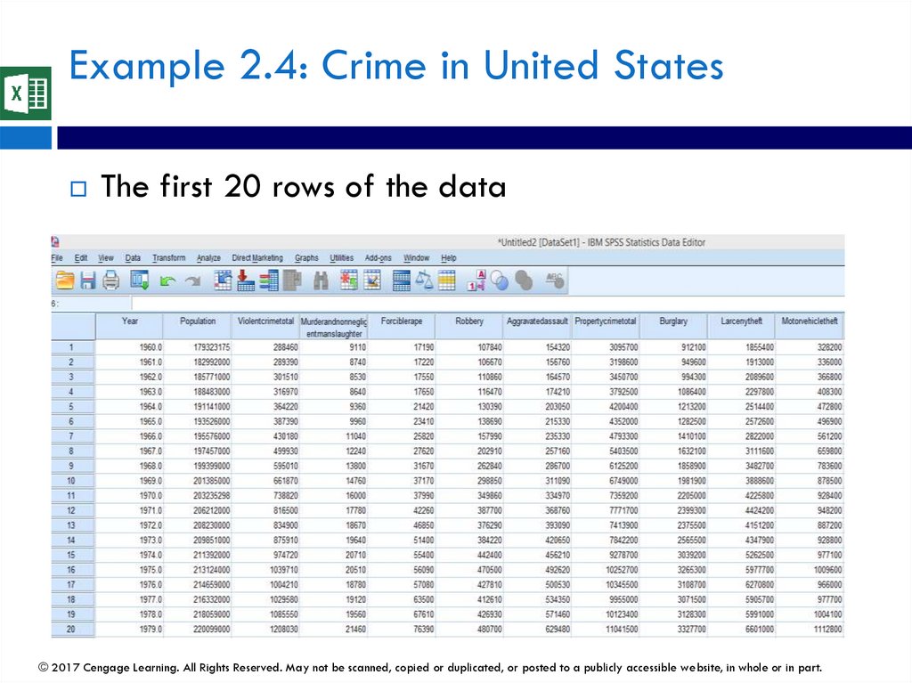
Example 2.4: Crime in United StatesThe first 20 rows of the data
© 2017 Cengage Learning. All Rights Reserved. May not be scanned, copied or duplicated, or posted to a publicly accessible website, in whole or in part.
157.
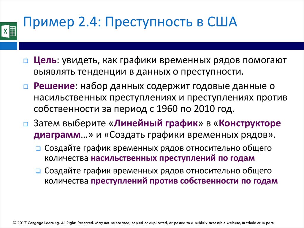
Пример 2.4: Преступность в СШАЦель: увидеть, как графики временных рядов помогают
выявлять тенденции в данных о преступности.
Решение: набор данных содержит годовые данные о
насильственных преступлениях и преступлениях против
собственности за период с 1960 по 2010 год.
Затем выберите «Линейный график» в «Конструкторе
диаграмм…» и «Создать графики временных рядов».
Создайте график временных рядов относительно общего
количества насильственных преступлений по годам
Создайте график временных рядов относительно общего
количества преступлений против собственности по годам
© 2017 Cengage Learning. All Rights Reserved. May not be scanned, copied or duplicated, or posted to a publicly accessible website, in whole or in part.
158.
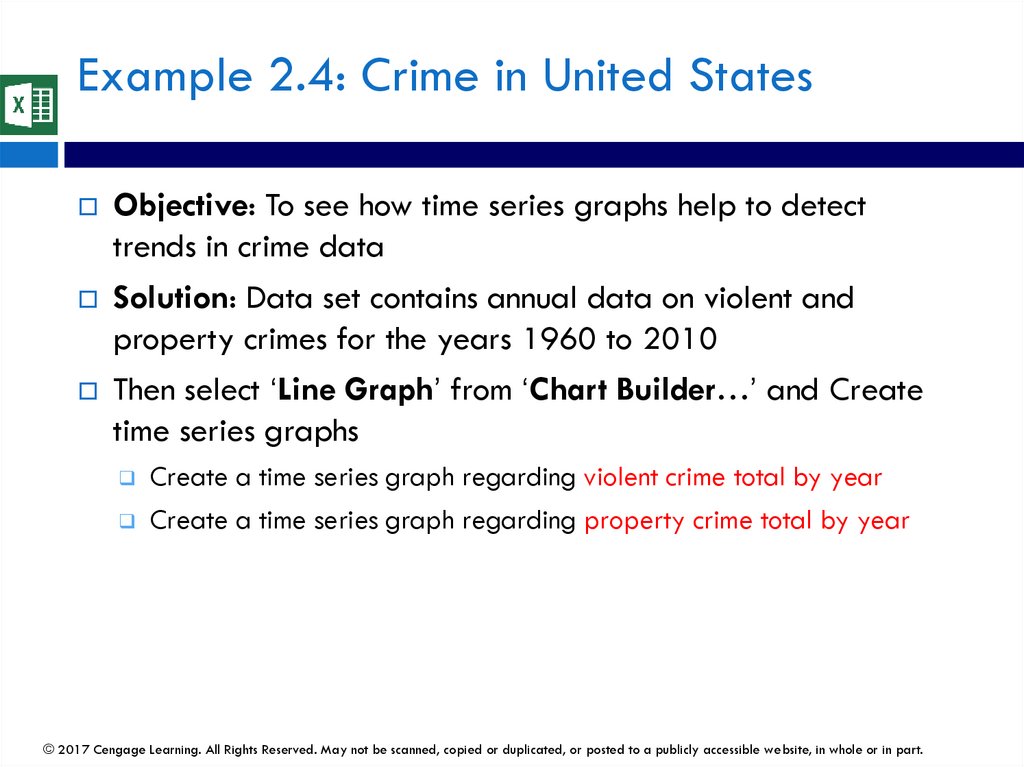
Example 2.4: Crime in United StatesObjective: To see how time series graphs help to detect
trends in crime data
Solution: Data set contains annual data on violent and
property crimes for the years 1960 to 2010
Then select ‘Line Graph’ from ‘Chart Builder…’ and Create
time series graphs
Create a time series graph regarding violent crime total by year
Create a time series graph regarding property crime total by year
© 2017 Cengage Learning. All Rights Reserved. May not be scanned, copied or duplicated, or posted to a publicly accessible website, in whole or in part.
159.
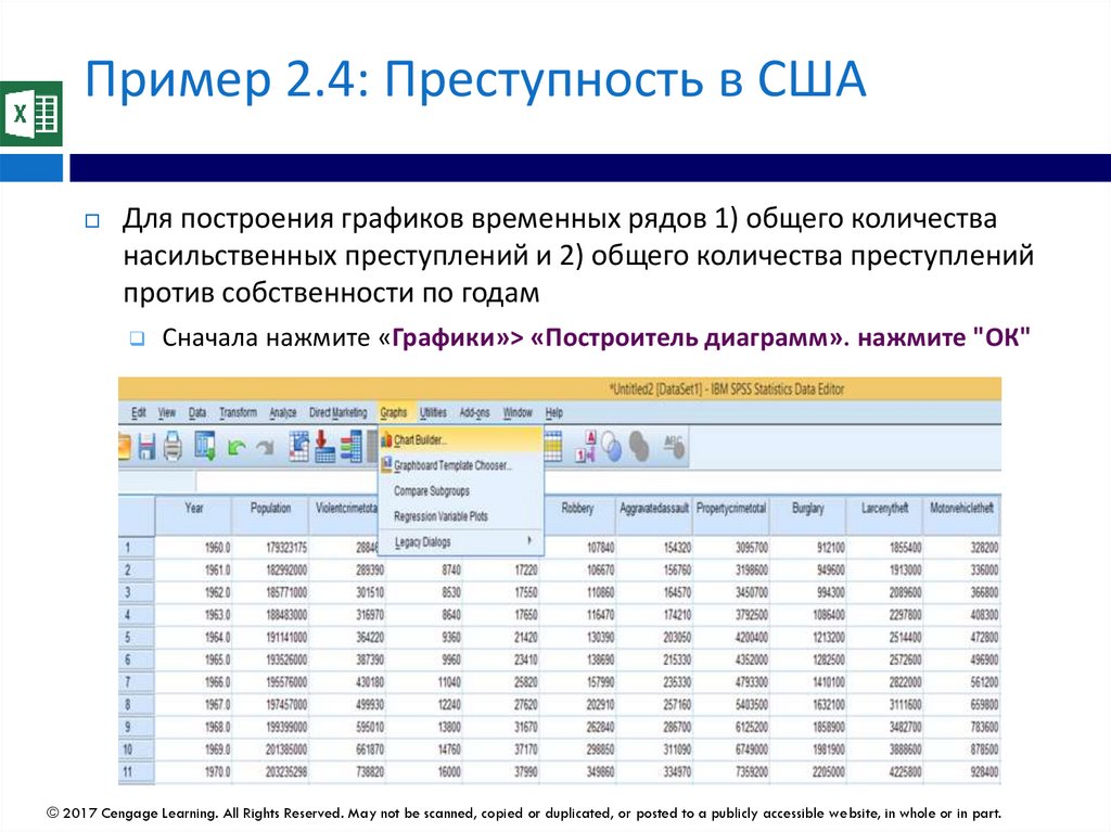
Пример 2.4: Преступность в СШАДля построения графиков временных рядов 1) общего количества
насильственных преступлений и 2) общего количества преступлений
против собственности по годам
Сначала нажмите «Графики»> «Построитель диаграмм». нажмите "ОК"
© 2017 Cengage Learning. All Rights Reserved. May not be scanned, copied or duplicated, or posted to a publicly accessible website, in whole or in part.
160.
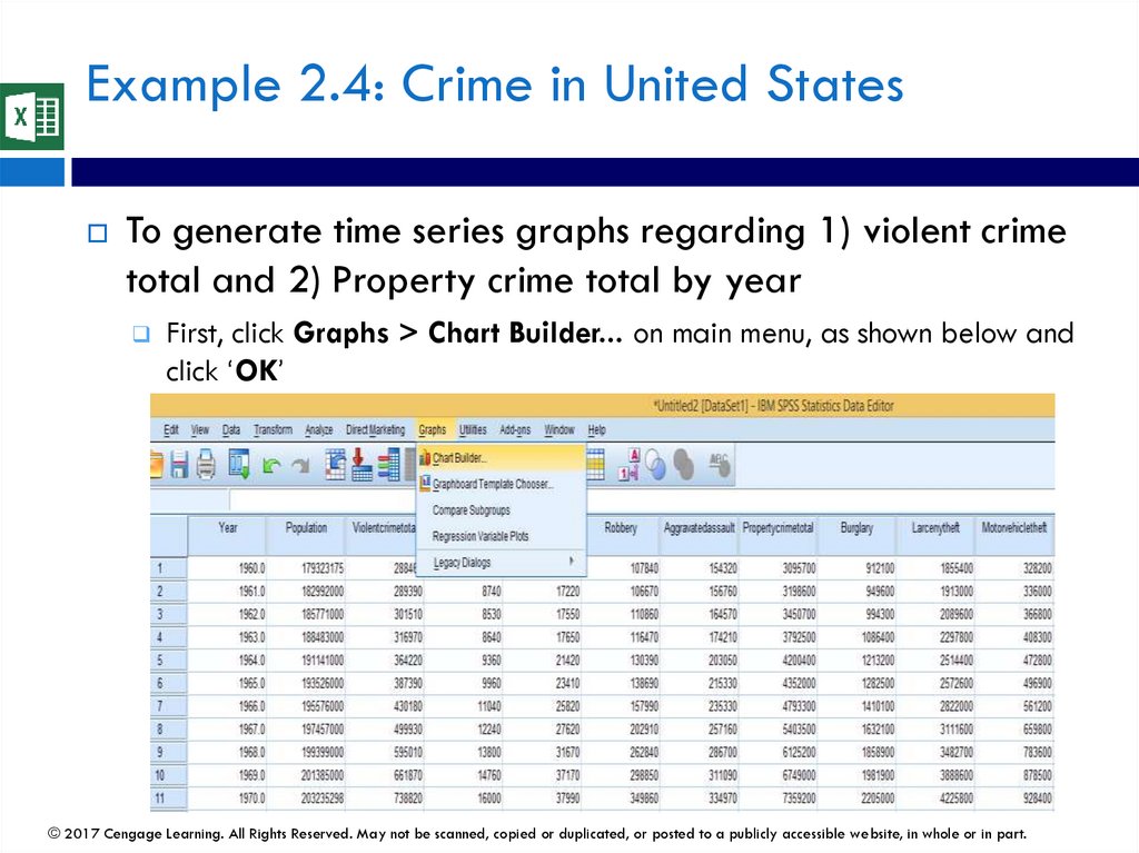
Example 2.4: Crime in United StatesTo generate time series graphs regarding 1) violent crime
total and 2) Property crime total by year
First, click Graphs > Chart Builder... on main menu, as shown below and
click ‘OK’
© 2017 Cengage Learning. All Rights Reserved. May not be scanned, copied or duplicated, or posted to a publicly accessible website, in whole or in part.
161.
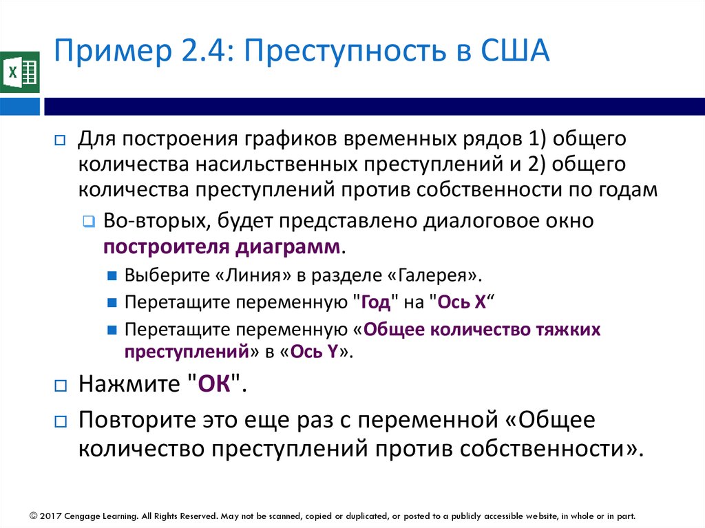
Пример 2.4: Преступность в СШАДля построения графиков временных рядов 1) общего
количества насильственных преступлений и 2) общего
количества преступлений против собственности по годам
Во-вторых, будет представлено диалоговое окно
построителя диаграмм.
Выберите «Линия» в разделе «Галерея».
Перетащите переменную "Год" на "Ось X“
Перетащите переменную «Общее количество тяжких
преступлений» в «Ось Y».
Нажмите "ОК".
Повторите это еще раз с переменной «Общее
количество преступлений против собственности».
© 2017 Cengage Learning. All Rights Reserved. May not be scanned, copied or duplicated, or posted to a publicly accessible website, in whole or in part.
162.
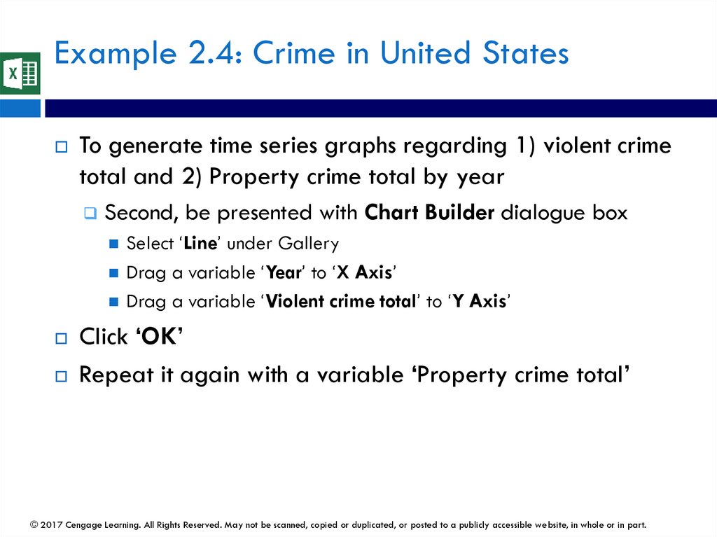
Example 2.4: Crime in United StatesTo generate time series graphs regarding 1) violent crime
total and 2) Property crime total by year
Second, be presented with Chart Builder dialogue box
Select ‘Line’ under Gallery
Drag a variable ‘Year’ to ‘X Axis’
Drag a variable ‘Violent crime total’ to ‘Y Axis’
Click ‘OK’
Repeat it again with a variable ‘Property crime total’
© 2017 Cengage Learning. All Rights Reserved. May not be scanned, copied or duplicated, or posted to a publicly accessible website, in whole or in part.
163.
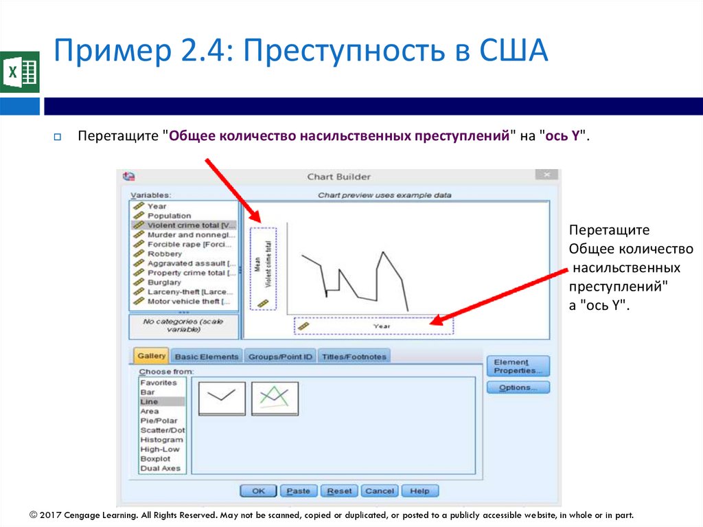
Пример 2.4: Преступность в СШАПеретащите "Общее количество насильственных преступлений" на "ось Y".
Перетащите
Общее количество
насильственных
преступлений"
а "ось Y".
© 2017 Cengage Learning. All Rights Reserved. May not be scanned, copied or duplicated, or posted to a publicly accessible website, in whole or in part.
164.
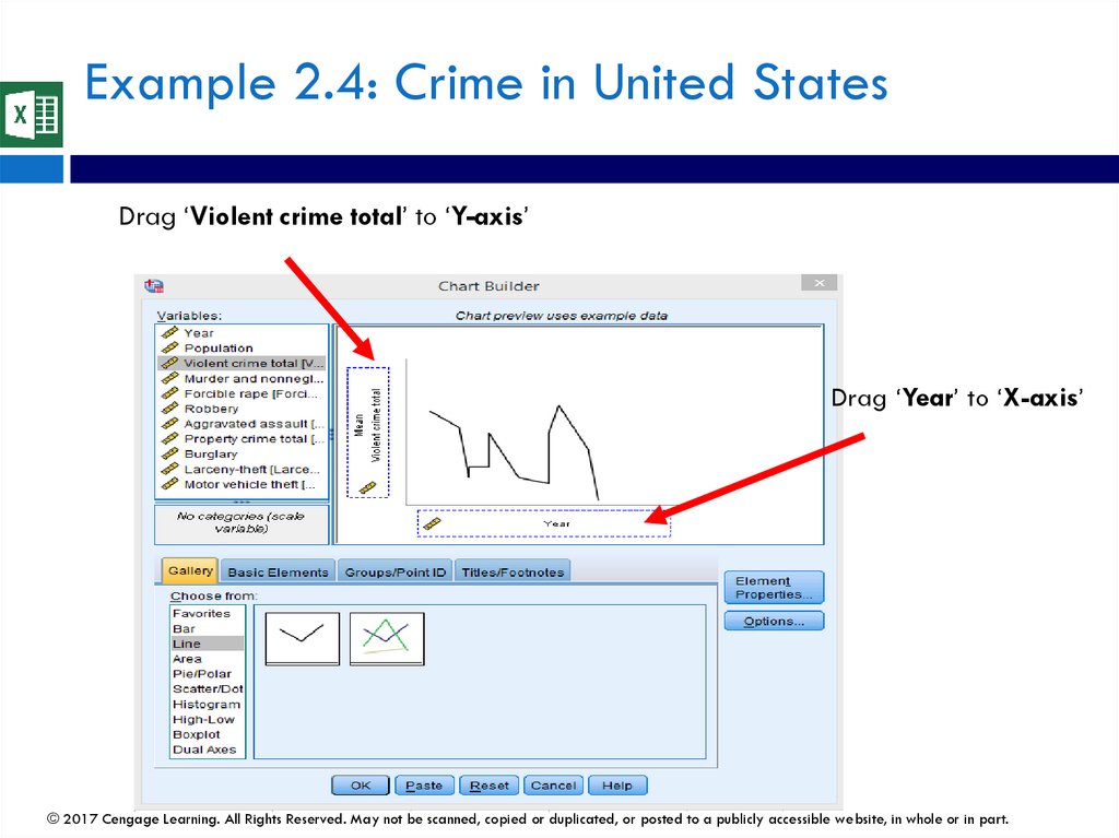
Example 2.4: Crime in United StatesDrag ‘Violent crime total’ to ‘Y-axis’
Drag ‘Year’ to ‘X-axis’
© 2017 Cengage Learning. All Rights Reserved. May not be scanned, copied or duplicated, or posted to a publicly accessible website, in whole or in part.
165.
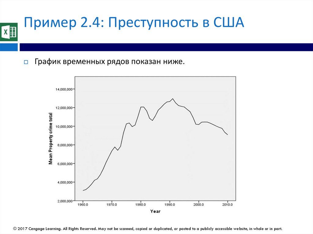
Пример 2.4: Преступность в СШАГрафик временных рядов показан ниже.
© 2017 Cengage Learning. All Rights Reserved. May not be scanned, copied or duplicated, or posted to a publicly accessible website, in whole or in part.
166.
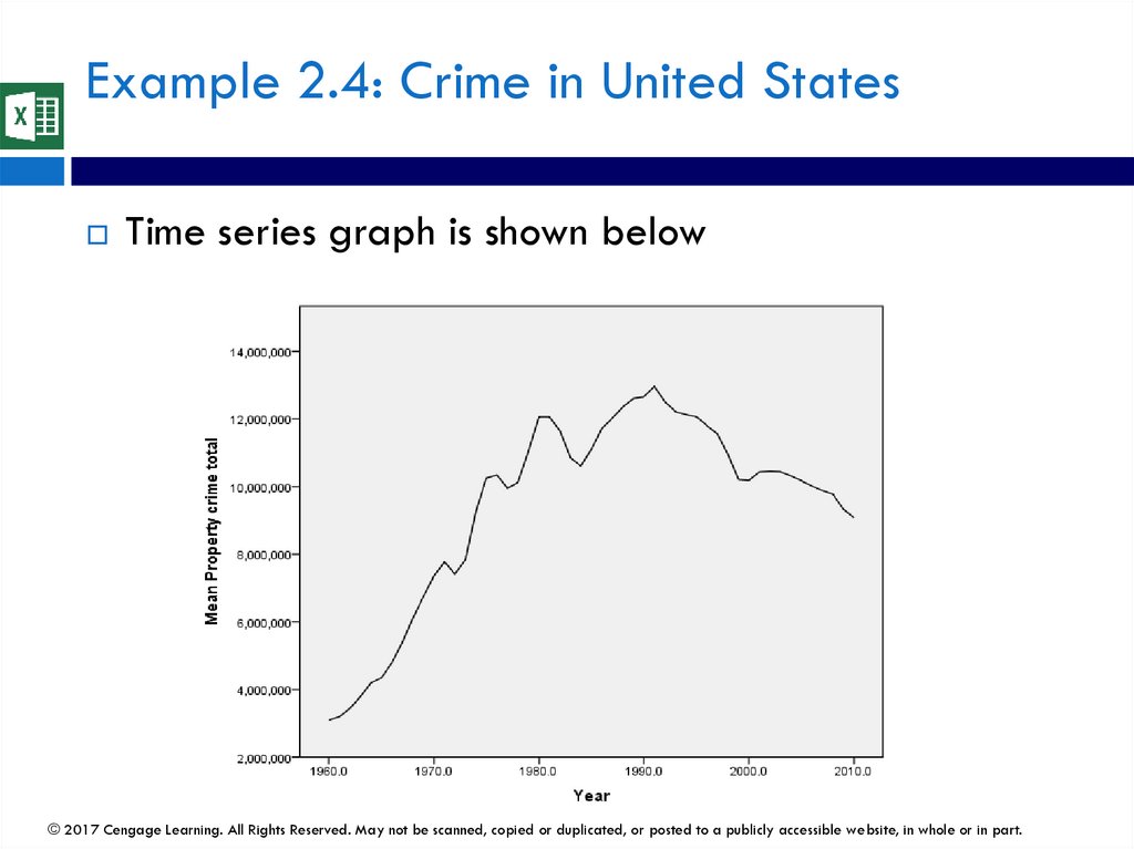
Example 2.4: Crime in United StatesTime series graph is shown below
© 2017 Cengage Learning. All Rights Reserved. May not be scanned, copied or duplicated, or posted to a publicly accessible website, in whole or in part.
167.
Классная работаСоздайте график временных рядов "Население"
по "годам"
© 2017 Cengage Learning. All Rights Reserved. May not be scanned, copied or duplicated, or posted to a publicly accessible website, in whole or in part.
168.
Class ExerciseGenerate a time series graph regarding ‘Population’
by ‘year’
© 2017 Cengage Learning. All Rights Reserved. May not be scanned, copied or duplicated, or posted to a publicly accessible website, in whole or in part.
169.
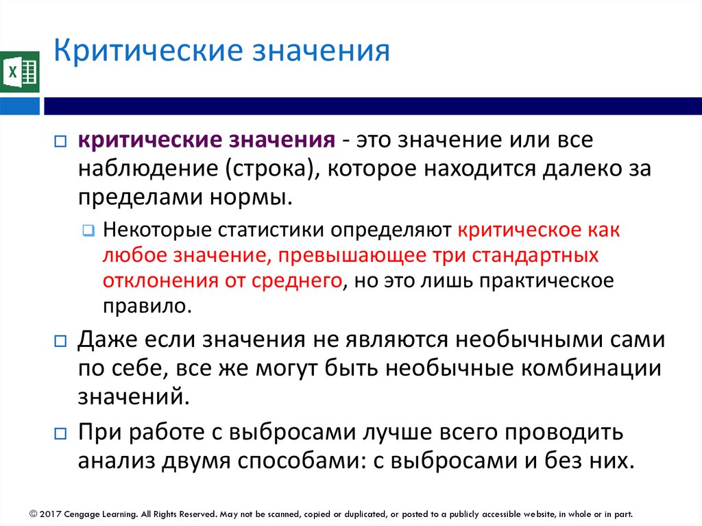
Критические значениякритические значения - это значение или все
наблюдение (строка), которое находится далеко за
пределами нормы.
Некоторые статистики определяют критическое как
любое значение, превышающее три стандартных
отклонения от среднего, но это лишь практическое
правило.
Даже если значения не являются необычными сами
по себе, все же могут быть необычные комбинации
значений.
При работе с выбросами лучше всего проводить
анализ двумя способами: с выбросами и без них.
© 2017 Cengage Learning. All Rights Reserved. May not be scanned, copied or duplicated, or posted to a publicly accessible website, in whole or in part.
170.
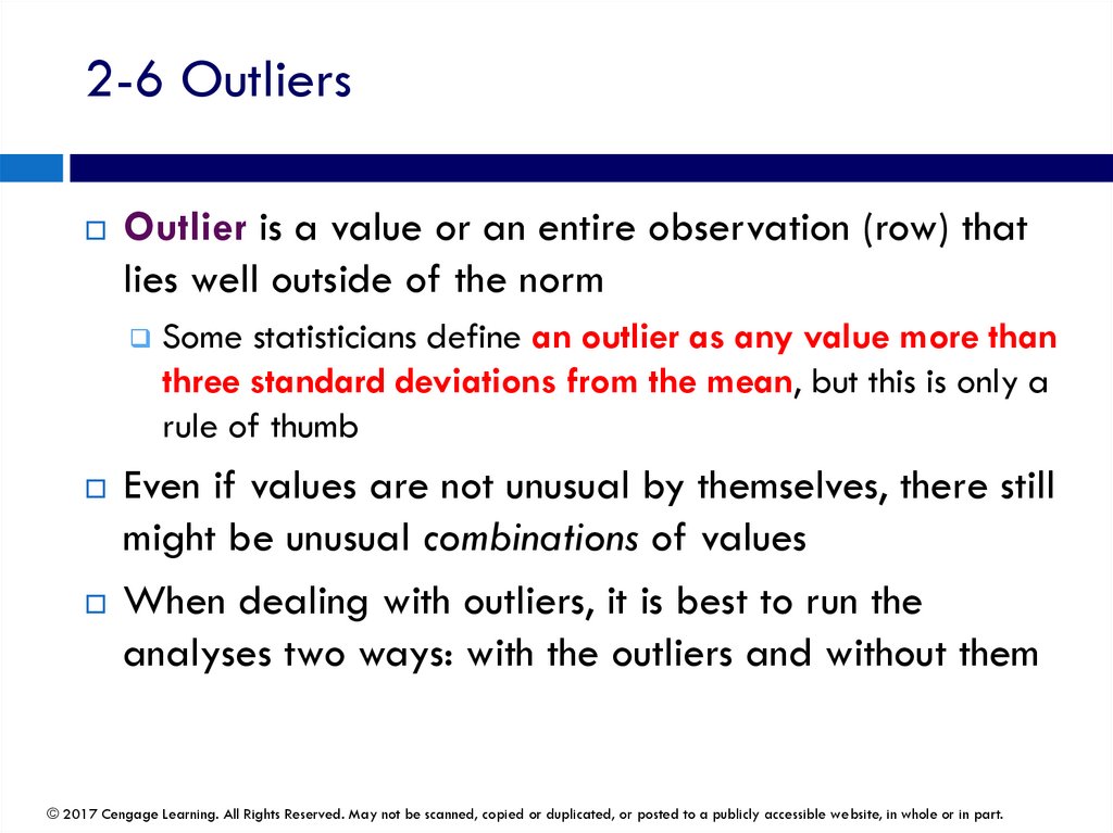
2-6 OutliersOutlier is a value or an entire observation (row) that
lies well outside of the norm
Some statisticians define an outlier as any value more than
three standard deviations from the mean, but this is only a
rule of thumb
Even if values are not unusual by themselves, there still
might be unusual combinations of values
When dealing with outliers, it is best to run the
analyses two ways: with the outliers and without them
© 2017 Cengage Learning. All Rights Reserved. May not be scanned, copied or duplicated, or posted to a publicly accessible website, in whole or in part.
171.
2-7 Фильтрация и сортировка в SPSSУдобный способ временно выбрать
подмножество наблюдений для анализа в SPSS использовать фильтр
Фильтрация - поиск записей, соответствующих
определенным критериям
У вас есть возможность назначить новый набор
данных в виде таблицы, а затем использовать
ряд мощных инструментов для анализа таблиц.
Эти инструменты включают:
Фильтрация
Сортировка
© 2017 Cengage Learning. All Rights Reserved. May not be scanned, copied or duplicated, or posted to a publicly accessible website, in whole or in part.
172.
2-7 Filtering and Sorting in SPSSA convenient way to temporarily select a subset of
case for analysis in SPSS is to use a filter
Filtering - Finding records that match particular criteria
You have the ability to designate a new data set as a
table and then employ a number of powerful tools
for analyzing tables
These tools include:
Filtering
Sorting
© 2017 Cengage Learning. All Rights Reserved. May not be scanned, copied or duplicated, or posted to a publicly accessible website, in whole or in part.
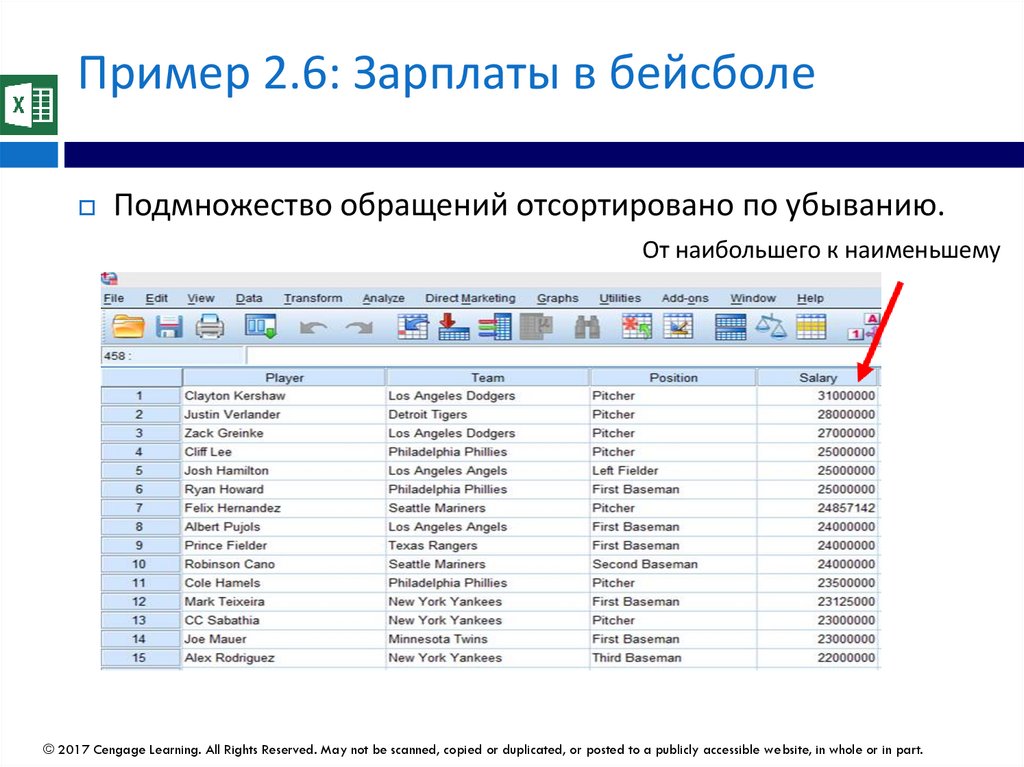
173.
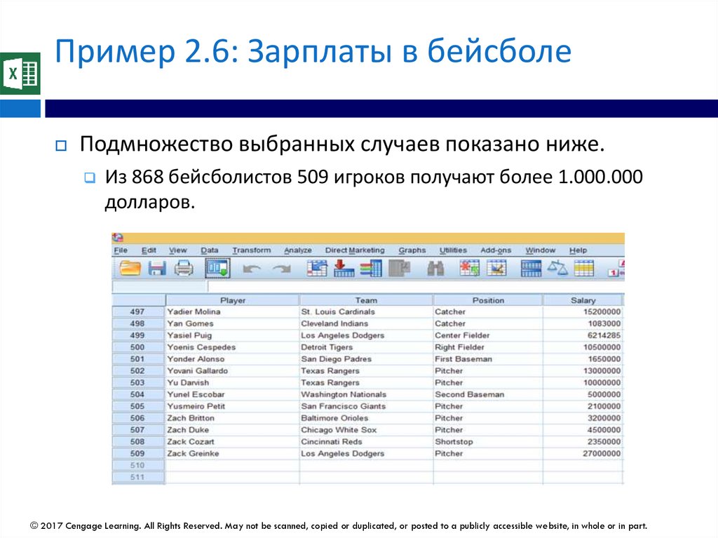
Пример 2.6: Зарплаты в бейсболеЦель: изучить типы фильтров, которые можно применить
к зарплате в бейсболе.
Решение: количество фильтров, которые вы можете
применять, почти не ограничено, но есть несколько
возможностей:
Мы хотим выбрать случаи, когда «зарплата равна или
превышает 1 000 000 долларов США».
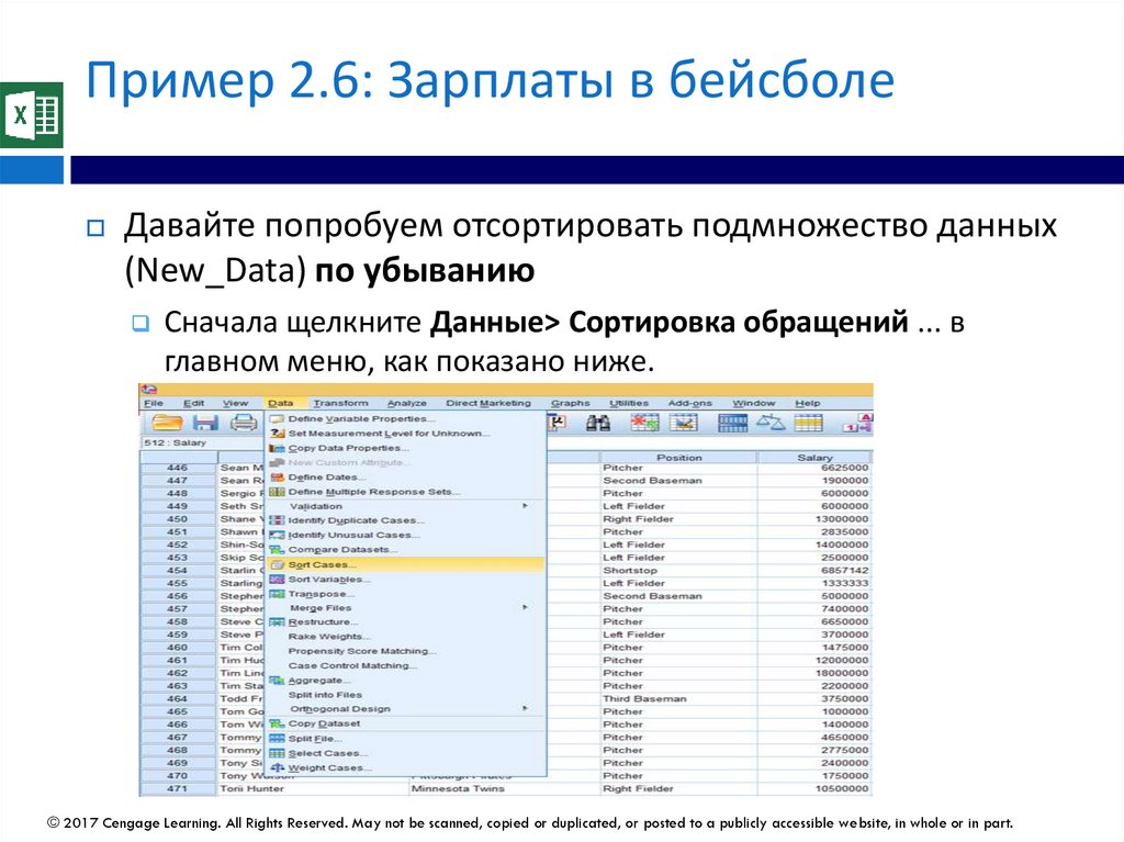
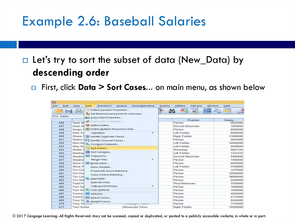
Мы хотим отсортировать подмножество обращений по
«убыванию» (от наибольшего к наименьшему)
© 2017 Cengage Learning. All Rights Reserved. May not be scanned, copied or duplicated, or posted to a publicly accessible website, in whole or in part.
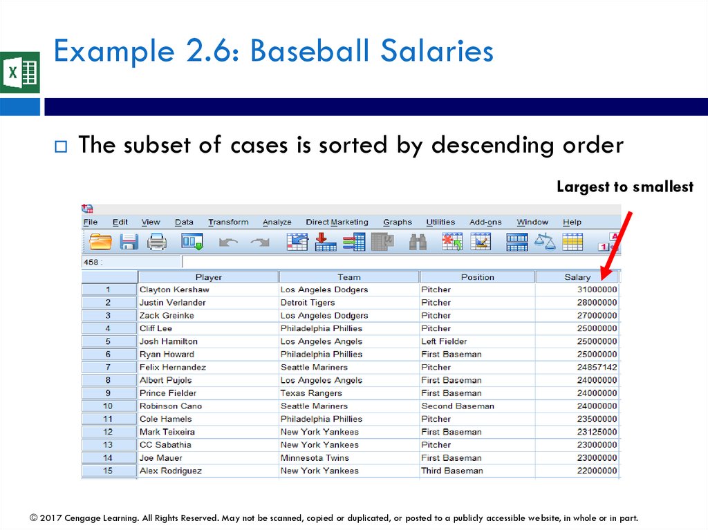
174.
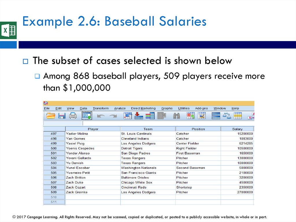
Example 2.6: Baseball SalariesObjective: To investigate the types of filters that can be
applied to the Baseball Salaries
Solution: There is almost no limit to the filters you can
apply, but here are a few possibilities:
We want to select cases where ‘salary is equal or greater than
$1,000,000’
We want to sort the subset of cases by ‘descending order’
(largest to smallest)
© 2017 Cengage Learning. All Rights Reserved. May not be scanned, copied or duplicated, or posted to a publicly accessible website, in whole or in part.
175.
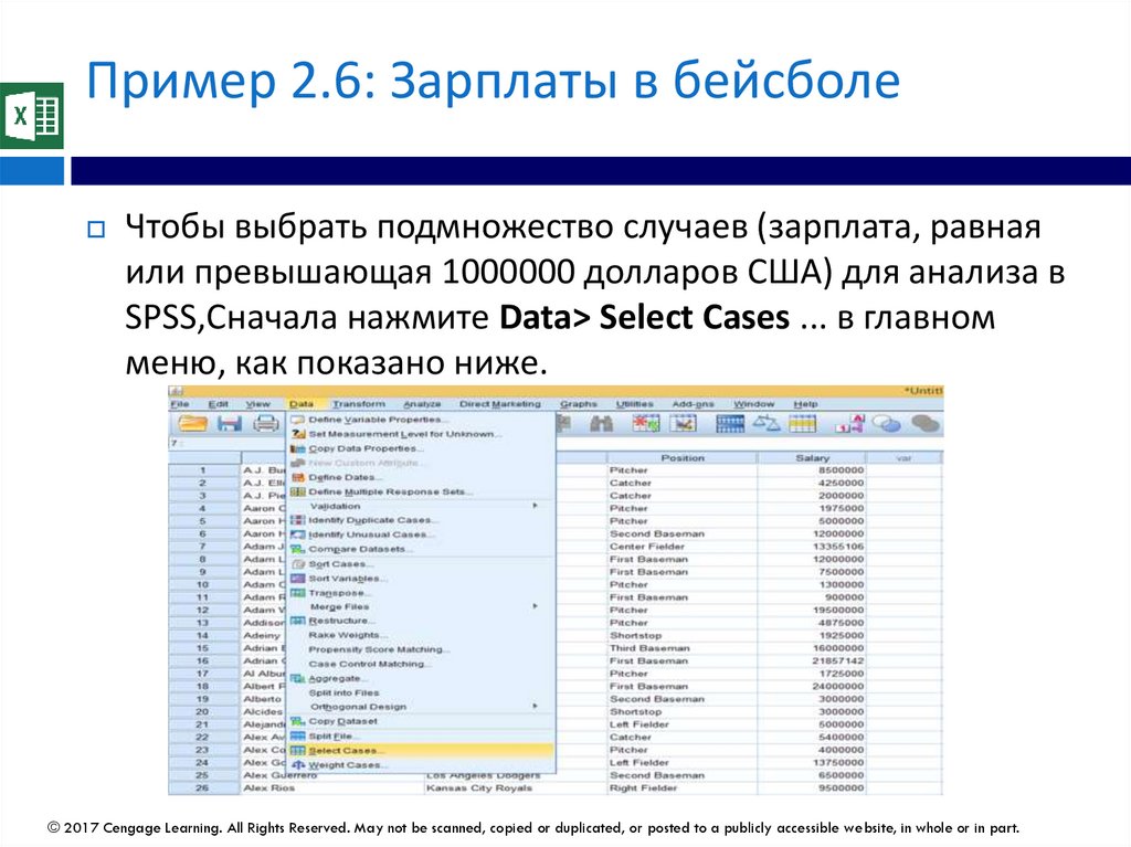
Пример 2.6: Зарплаты в бейсболеЧтобы выбрать подмножество случаев (зарплата, равная
или превышающая 1000000 долларов США) для анализа в
SPSS,Сначала нажмите Data> Select Cases ... в главном
меню, как показано ниже.
© 2017 Cengage Learning. All Rights Reserved. May not be scanned, copied or duplicated, or posted to a publicly accessible website, in whole or in part.
176.
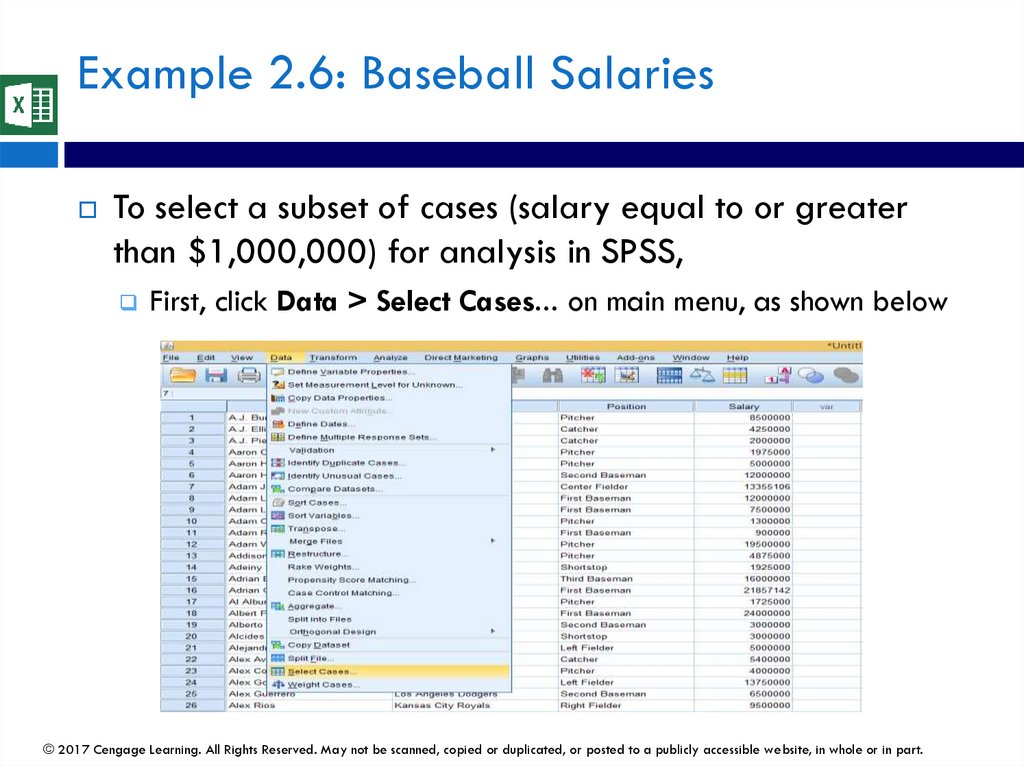
Example 2.6: Baseball SalariesTo select a subset of cases (salary equal to or greater
than $1,000,000) for analysis in SPSS,
First, click Data > Select Cases... on main menu, as shown below
© 2017 Cengage Learning. All Rights Reserved. May not be scanned, copied or duplicated, or posted to a publicly accessible website, in whole or in part.
177.
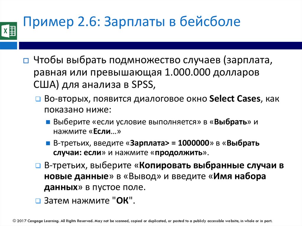
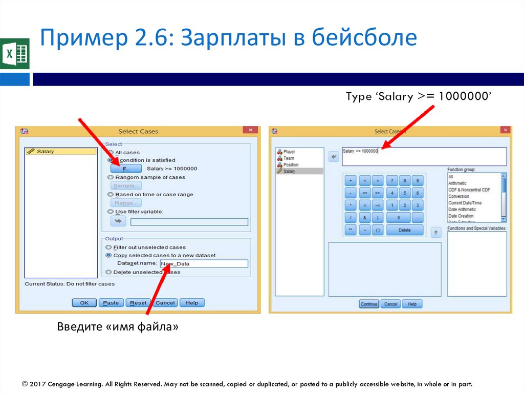
Пример 2.6: Зарплаты в бейсболеЧтобы выбрать подмножество случаев (зарплата,
равная или превышающая 1.000.000 долларов
США) для анализа в SPSS,
Во-вторых, появится диалоговое окно Select Cases, как
показано ниже:
Выберите «если условие выполняется» в «Выбрать» и
нажмите «Если…»
В-третьих, введите «Зарплата> = 1000000» в «Выбрать
случаи: если» и нажмите «продолжить».
В-третьих, выберите «Копировать выбранные случаи в
новые данные» в «Вывод» и введите «Имя набора
данных» в пустое поле.
Затем нажмите "ОК".
© 2017 Cengage Learning. All Rights Reserved. May not be scanned, copied or duplicated, or posted to a publicly accessible website, in whole or in part.
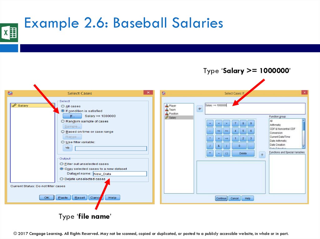
178.
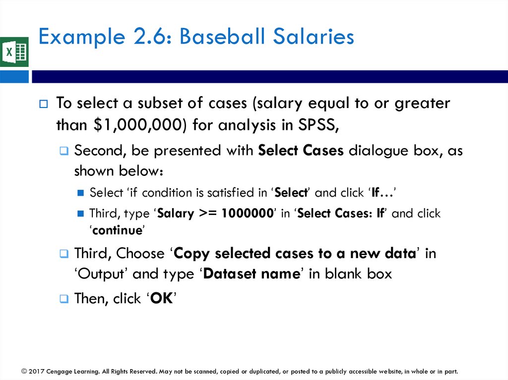
Example 2.6: Baseball SalariesTo select a subset of cases (salary equal to or greater
than $1,000,000) for analysis in SPSS,
Second, be presented with Select Cases dialogue box, as
shown below:
Select ‘if condition is satisfied in ‘Select’ and click ‘If…’
Third, type ‘Salary >= 1000000’ in ‘Select Cases: If’ and click
‘continue’
Third, Choose ‘Copy selected cases to a new data’ in
‘Output’ and type ‘Dataset name’ in blank box
Then, click ‘OK’
© 2017 Cengage Learning. All Rights Reserved. May not be scanned, copied or duplicated, or posted to a publicly accessible website, in whole or in part.
179.
Пример 2.6: Зарплаты в бейсболеType ‘Salary >= 1000000’
Введите «имя файла»
© 2017 Cengage Learning. All Rights Reserved. May not be scanned, copied or duplicated, or posted to a publicly accessible website, in whole or in part.
180.
Example 2.6: Baseball SalariesType ‘Salary >= 1000000’
Type ‘file name’
© 2017 Cengage Learning. All Rights Reserved. May not be scanned, copied or duplicated, or posted to a publicly accessible website, in whole or in part.
181.
Пример 2.6: Зарплаты в бейсболеПодмножество выбранных случаев показано ниже.
Из 868 бейсболистов 509 игроков получают более 1.000.000
долларов.
© 2017 Cengage Learning. All Rights Reserved. May not be scanned, copied or duplicated, or posted to a publicly accessible website, in whole or in part.
182.
Example 2.6: Baseball SalariesThe subset of cases selected is shown below
Among 868 baseball players, 509 players receive more
than $1,000,000
© 2017 Cengage Learning. All Rights Reserved. May not be scanned, copied or duplicated, or posted to a publicly accessible website, in whole or in part.
183.
Пример 2.6: Зарплаты в бейсболеДавайте попробуем отсортировать подмножество данных
(New_Data) по убыванию
Сначала щелкните Данные> Сортировка обращений ... в
главном меню, как показано ниже.
© 2017 Cengage Learning. All Rights Reserved. May not be scanned, copied or duplicated, or posted to a publicly accessible website, in whole or in part.
184.
Example 2.6: Baseball SalariesLet’s try to sort the subset of data (New_Data) by
descending order
First, click Data > Sort Cases... on main menu, as shown below
© 2017 Cengage Learning. All Rights Reserved. May not be scanned, copied or duplicated, or posted to a publicly accessible website, in whole or in part.
185.
Пример 2.6: Зарплаты в бейсболеВо-вторых, появится диалоговое окно «Сортировка дел», как
показано ниже:
Перетащите «Зарплата» в поле «Сортировать по:».
Выберите «По убыванию» в разделе «Сортировка по одеру».
Затем нажмите "ОК".
© 2017 Cengage Learning. All Rights Reserved. May not be scanned, copied or duplicated, or posted to a publicly accessible website, in whole or in part.
186.
Example 2.6: Baseball SalariesSecond, be presented with the Sort Cases dialogue box, as
shown below:
Drag ‘Salary’ to ‘Sort by:’ Box
Choose ‘Descending’ in Sort Oder
Then, click ‘OK’
© 2017 Cengage Learning. All Rights Reserved. May not be scanned, copied or duplicated, or posted to a publicly accessible website, in whole or in part.
187.
Пример 2.6: Зарплаты в бейсболеПодмножество обращений отсортировано по убыванию.
От наибольшего к наименьшему
© 2017 Cengage Learning. All Rights Reserved. May not be scanned, copied or duplicated, or posted to a publicly accessible website, in whole or in part.
188.
Example 2.6: Baseball SalariesThe subset of cases is sorted by descending order
Largest to smallest
© 2017 Cengage Learning. All Rights Reserved. May not be scanned, copied or duplicated, or posted to a publicly accessible website, in whole or in part.
189.
Классная упражнениеВыберите случаи, когда «зарплата равна или
превышает 5 000 000 долларов США»
Затем отсортируйте подмножество выбранных
обращений по «возрастанию».
© 2017 Cengage Learning. All Rights Reserved. May not be scanned, copied or duplicated, or posted to a publicly accessible website, in whole or in part.
190.
Class ExercisePlease select cases where ‘salary is equal or
greater than $5,000,000’
Then, sort the subset of selected cases by
‘ascending order’
© 2017 Cengage Learning. All Rights Reserved. May not be scanned, copied or duplicated, or posted to a publicly accessible website, in whole or in part.