Machine Learning Foundations for Product Managers

1.

Machine Learning Foundations for
Product Managers
Peer-graded Assignment: Course Project.

2.

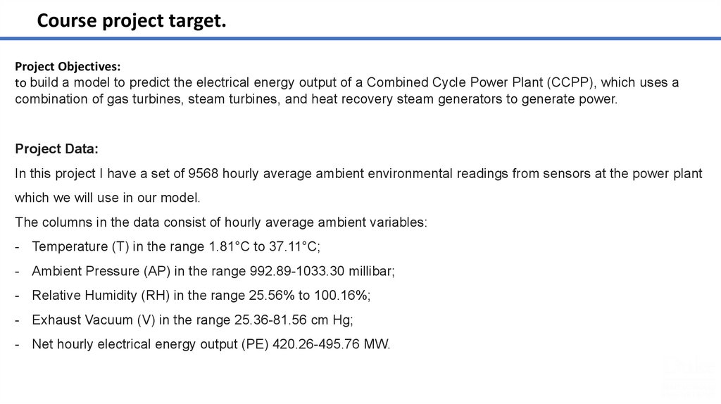
Course project target.
Project Objectives:
to build a model to predict the electrical energy output of a Combined Cycle Power Plant (CCPP), which uses a
combination of gas turbines, steam turbines, and heat recovery steam generators to generate power.
Project Data:
In this project I have a set of 9568 hourly average ambient environmental readings from sensors at the power plant
which we will use in our model.
The columns in the data consist of hourly average ambient variables:
- Temperature (T) in the range 1.81°C to 37.11°C;
- Ambient Pressure (AP) in the range 992.89-1033.30 millibar;
- Relative Humidity (RH) in the range 25.56% to 100.16%;
- Exhaust Vacuum (V) in the range 25.36-81.56 cm Hg;
- Net hourly electrical energy output (PE) 420.26-495.76 MW.

3.

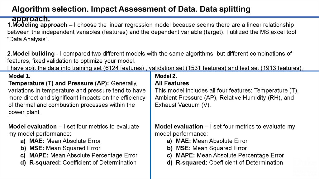
Algorithm selection. Impact Assessment of Data. Data splitting
approach.
1.Modeling approach – I choose the linear regression model because seems there are a linear relationship
between the independent variables (features) and the dependent variable (target). I utilized the MS excel tool
“Data Analysis”.
2.Model building - I compared two different models with the same algorithms, but different combinations of
features, fixed validation to optimize your model.
I have split the data into training set (6124 features) , validation set (1531 features) and test set (1913 features),
Model 1.
Model 2.
Temperature (T) and Pressure (AP): Generally,
All Features
variations in temperature and pressure tend to have
This model includes all four features: Temperature (T),
more direct and significant impacts on the efficiency
Ambient Pressure (AP), Relative Humidity (RH), and
of thermal and combustion processes within the
Exhaust Vacuum (V).
power plant.
Model evaluation – I set four metrics to evaluate
my model performance:
a) MAE: Mean Absolute Error
b) MSE: Mean Squared Error
c) MAPE: Mean Absolute Percentage Error
d) R-squared: Coefficient of Determination
Model evaluation – I set four metrics to evaluate my
model performance:
a) MAE: Mean Absolute Error
b) MSE: Mean Squared Error
c) MAPE: Mean Absolute Percentage Error
d) R-squared: Coefficient of Determination

4.

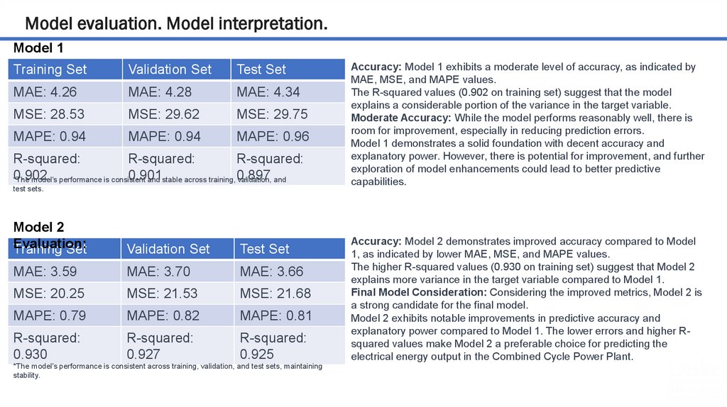
Model evaluation. Model interpretation.
Model 1
Evaluation:
Training Set
Validation Set
Test Set
MAE: 4.26
MAE: 4.28
MAE: 4.34
MSE: 28.53
MSE: 29.62
MSE: 29.75
MAPE: 0.94
MAPE: 0.94
MAPE: 0.96
R-squared:
R-squared:
R-squared:
0.902
0.901
*The model's performance is consistent
and stable across training, 0.897
validation, and
test sets.
Model 2
Evaluation:
Training Set
Validation Set
Test Set
MAE: 3.59
MAE: 3.70
MAE: 3.66
MSE: 20.25
MSE: 21.53
MSE: 21.68
MAPE: 0.79
MAPE: 0.82
MAPE: 0.81
R-squared:
0.930
R-squared:
0.927
R-squared:
0.925
*The model's performance is consistent across training, validation, and test sets, maintaining
stability.
Accuracy: Model 1 exhibits a moderate level of accuracy, as indicated by
MAE, MSE, and MAPE values.
The R-squared values (0.902 on training set) suggest that the model
explains a considerable portion of the variance in the target variable.
Moderate Accuracy: While the model performs reasonably well, there is
room for improvement, especially in reducing prediction errors.
Model 1 demonstrates a solid foundation with decent accuracy and
explanatory power. However, there is potential for improvement, and further
exploration of model enhancements could lead to better predictive
capabilities.
Accuracy: Model 2 demonstrates improved accuracy compared to Model
1, as indicated by lower MAE, MSE, and MAPE values.
The higher R-squared values (0.930 on training set) suggest that Model 2
explains more variance in the target variable compared to Model 1.
Final Model Consideration: Considering the improved metrics, Model 2 is
a strong candidate for the final model.
Model 2 exhibits notable improvements in predictive accuracy and
explanatory power compared to Model 1. The lower errors and higher Rsquared values make Model 2 a preferable choice for predicting the
electrical energy output in the Combined Cycle Power Plant.