Индексирование, программирование, векторизация, графические возможности MatLab

1. Индексирование, программирование, векторизация, графические возможности MatLab

Лекция 3-4

2. Vector Indexing

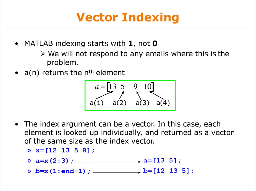
• MATLAB indexing starts with 1, not 0
We will not respond to any emails where this is the
problem.
• a(n) returns the nth element
a 13 5
a(1)
a(2)
9 10
a(3)
a(4)
• The index argument can be a vector. In this case, each
element is looked up individually, and returned as a vector
of the same size as the index vector.
» x=[12 13 5 8];
a=[13 5];
» a=x(2:3);
b=[12 13 5];
» b=x(1:end-1);

3. Matrix Indexing

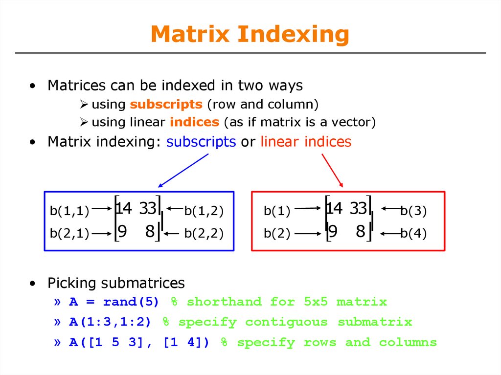
• Matrices can be indexed in two ways
using subscripts (row and column)
using linear indices (as if matrix is a vector)
• Matrix indexing: subscripts or linear indices
b(1,1)
b(2,1)
1
⎡ 4 33⎤
⎢9 8 ⎥
⎣
⎦
b(1,2)
b(1)
b(2,2)
b(2)
1
⎡ 4 33⎤
⎢9 8 ⎥
⎣
⎦
b(3)
b(4)
• Picking submatrices
» A = rand(5) % shorthand for 5x5 matrix
» A(1:3,1:2) % specify contiguous submatrix
» A([1 5 3], [1 4]) % specify rows and columns

4. Advanced Indexing 1

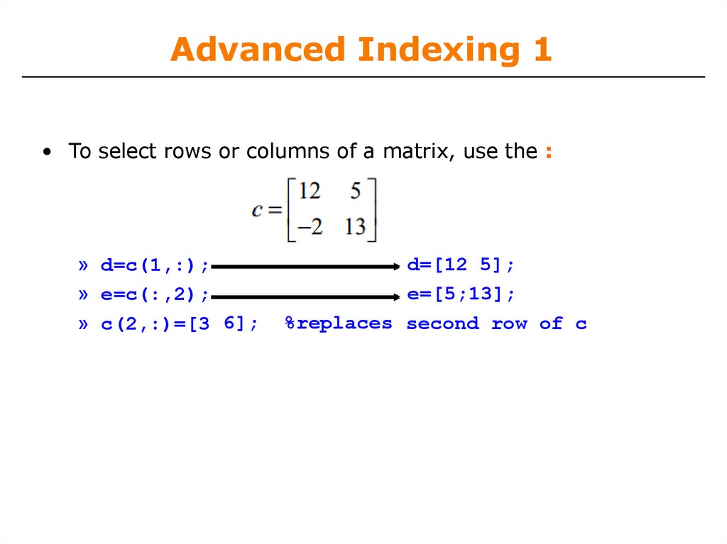
• To select rows or columns of a matrix, use the :
⎥
» d=c(1,:);
» e=c(:,2);
» c(2,:)=[3 6];
d=[12 5];
e=[5;13];
%replaces second row of c

5. Advanced Indexing 2

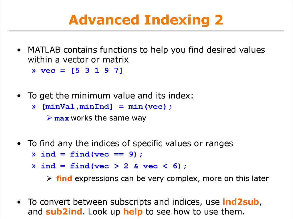
• MATLAB contains functions to help you find desired values
within a vector or matrix
» vec = [5 3 1 9 7]
• To get the minimum value and its index:
» [minVal,minInd] = min(vec);
max works the same way
• To find any the indices of specific values or ranges
» ind = find(vec == 9);
» ind = find(vec > 2 & vec < 6);
find expressions can be very complex, more on this later
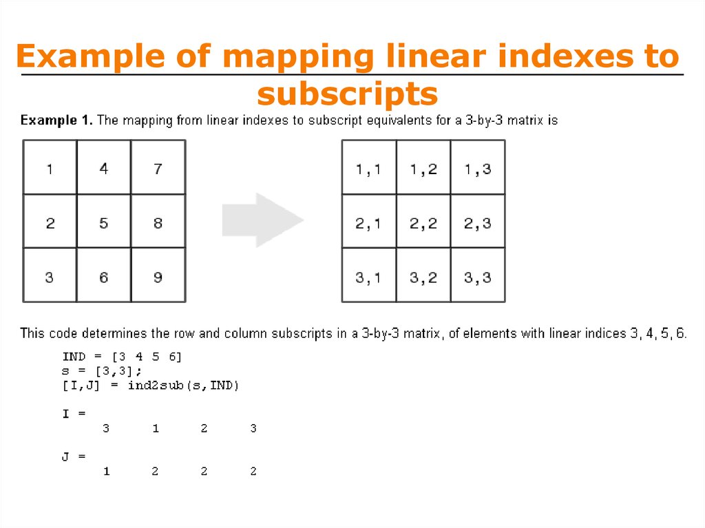
• To convert between subscripts and indices, use ind2sub,
and sub2ind. Look up help to see how to use them.

6. Example of mapping linear indexes to subscripts

7. Использование векторориентированных функций (max, min, sort, sum, mean, prod и других) с матричным аргументом

В случае с матрицами, функция max определяет
максимальные значения, стоящие в столбцах :
A = [4 3 5; 6 7 2; 3 1 8];
[V, I] = max(A);
% V=[6 7 8], I = [2 2 3]
V = max(A);
% V=[6 7 8]
Для поиска максимального значения во всей
матрице необходимо вызвать функцию дважды:
M = max(max(A));

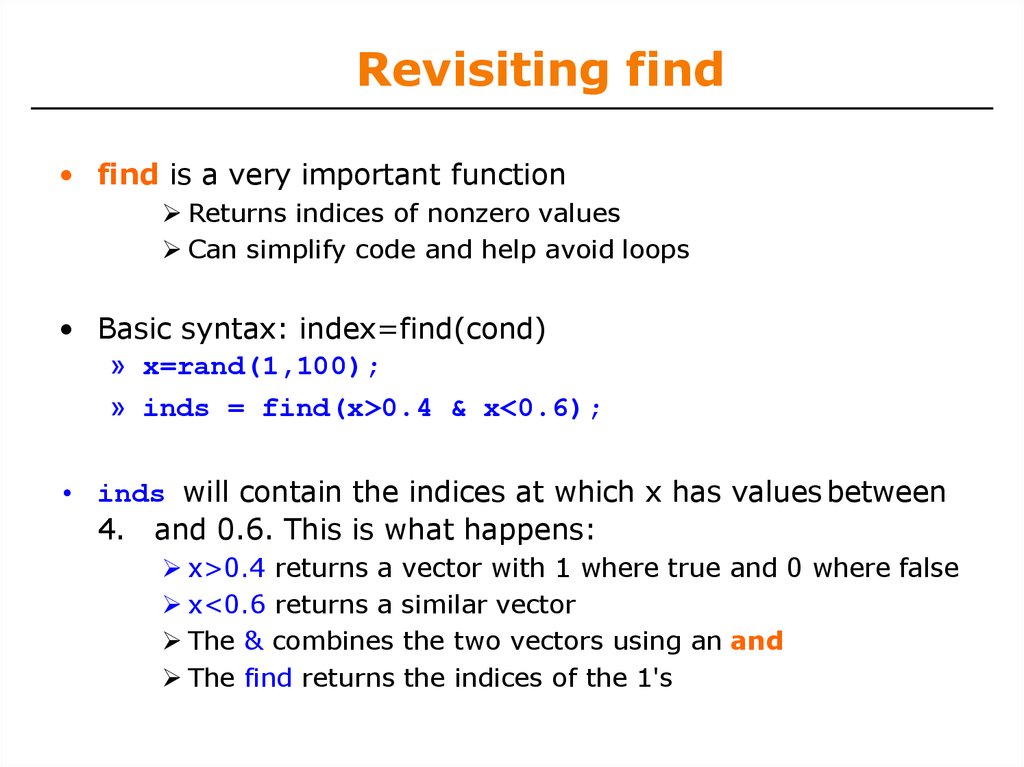
8. Revisiting find

• find is a very important function
Returns indices of nonzero values
Can simplify code and help avoid loops
• Basic syntax: index=find(cond)
» x=rand(1,100);
» inds = find(x>0.4 & x<0.6);
• inds will contain the indices at which x has values between
4. and 0.6. This is what happens:
x>0.4 returns a vector with 1 where true and 0 where false
x<0.6 returns a similar vector
The & combines the two vectors using an and
The find returns the indices of the 1's

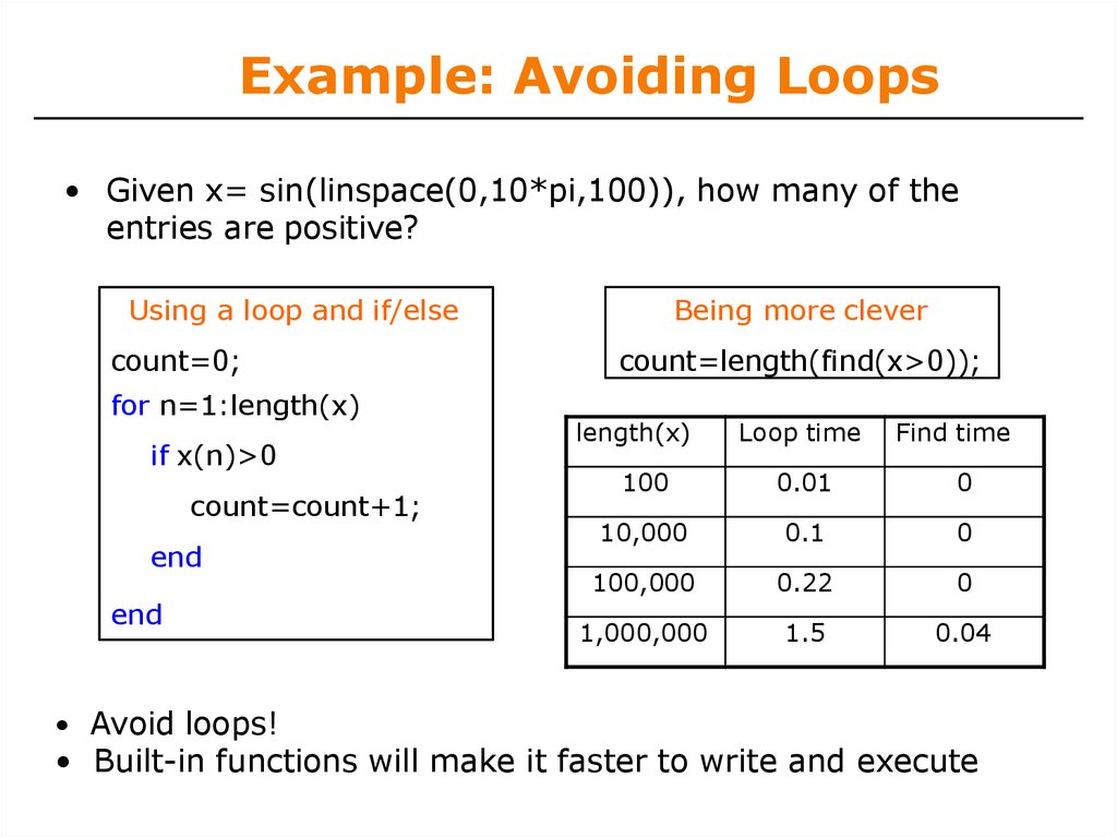
9. Example: Avoiding Loops

• Given x= sin(linspace(0,10*pi,100)), how many of the
entries are positive?
Using a loop and if/else
count=0;
for n=1:length(x)
if x(n)>0
count=count+1;
end
end
• Avoid loops!
Being more clever
count=length(find(x>0));
length(x)
Loop time
Find time
100
0.01
0
10,000
0.1
0
100,000
0.22
0
1,000,000
1.5
0.04
• Built-in functions will make it faster to write and execute

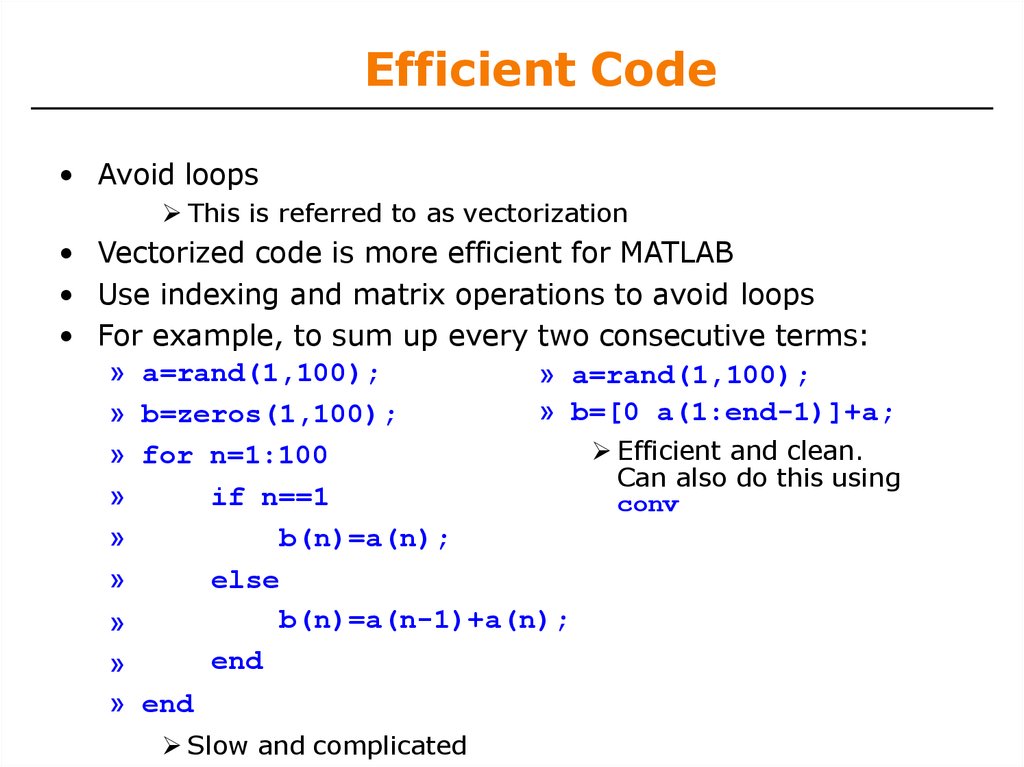
10. Efficient Code

• Avoid loops
This is referred to as vectorization
• Vectorized code is more efficient for MATLAB
• Use indexing and matrix operations to avoid loops
• For example, to sum up every two consecutive terms:
» a=rand(1,100);
» a=rand(1,100);
» b=[0 a(1:end-1)]+a;
» b=zeros(1,100);
Efficient and clean.
» for n=1:100
Can also do this using
»
if n==1
conv
»
b(n)=a(n);
»
else
b(n)=a(n-1)+a(n);
»
end
»
» end
Slow and complicated

11.

Vectorization makes
coding fun!

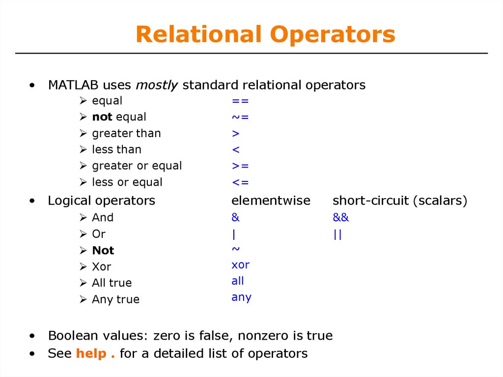
12. Relational Operators

• MATLAB uses mostly standard relational operators
equal
not equal
greater than
less than
greater or equal
less or equal
• Logical operators
And
Or
Not
Xor
All true
Any true
==
~=
>
<
>=
<=
elementwise
short-circuit (scalars)
&
|
~
xor
all
any
&&
||
• Boolean values: zero is false, nonzero is true
• See help . for a detailed list of operators

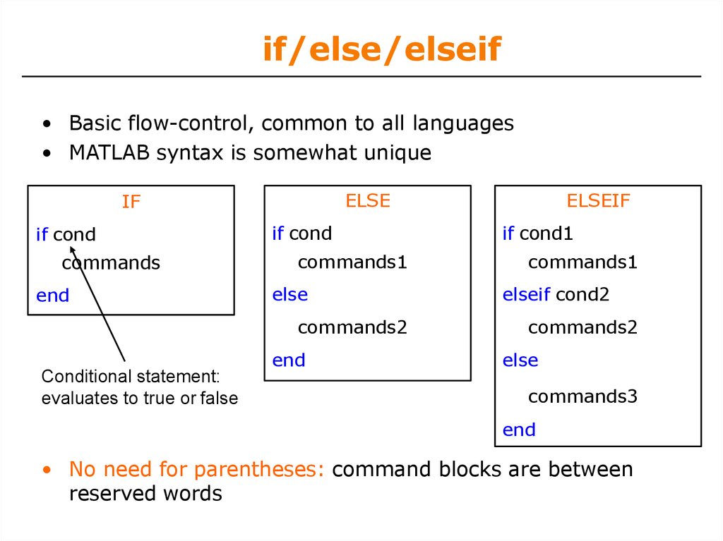
13. if/else/elseif

• Basic flow-control, common to all languages
• MATLAB syntax is somewhat unique
ELSE
IF
if cond
commands
end
if cond
commands1
else
commands2
Conditional statement:
evaluates to true or false
end
ELSEIF
if cond1
commands1
elseif cond2
commands2
else
commands3
end
• No need for parentheses: command blocks are between
reserved words

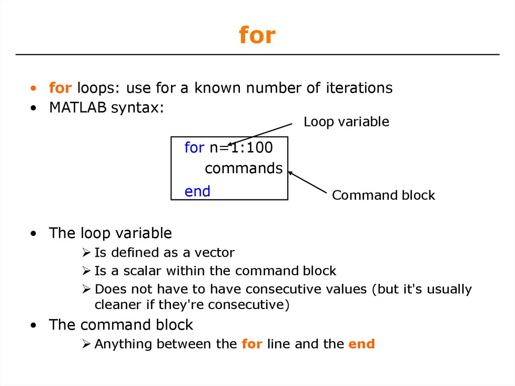
14. for loops: use for a known number of iterations

for
• for loops: use for a known number of iterations
• MATLAB syntax:
Loop variable
for n=1:100
commands
end
Command block
• The loop variable
Is defined as a vector
Is a scalar within the command block
Does not have to have consecutive values (but it's usually
cleaner if they're consecutive)
• The command block
Anything between the for line and the end

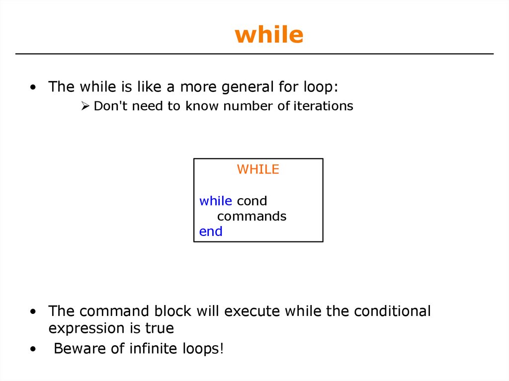
15. while

• The while is like a more general for loop:
Don't need to know number of iterations
WHILE
while cond
commands
end
• The command block will execute while the conditional
expression is true
• Beware of infinite loops!

16. Outline

(1)
(2)
(3)
(4)
(5)
Functions
Flow Control
Line Plots
Image/Surface Plots
Vectorization

17. User-defined Functions

• Functions look exactly like scripts, but for ONE difference
Functions must have a function declaration
Help file
Function declaration
Outputs
Inputs
Courtesy of The MathWorks, Inc. Used with permission.

18. User-defined Functions

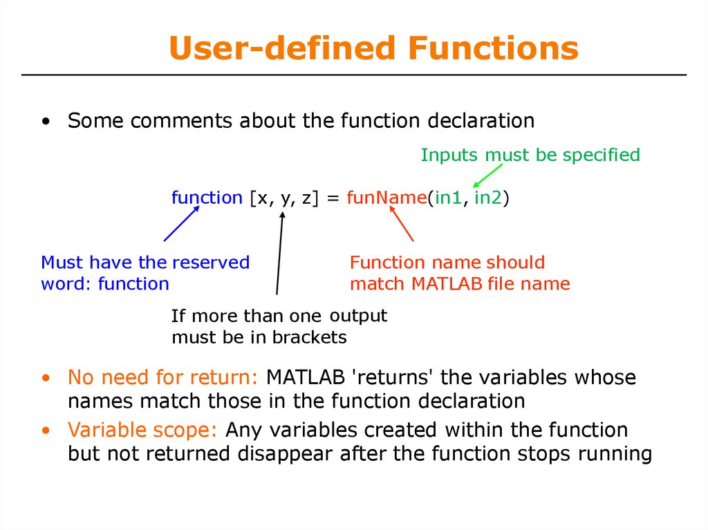
• Some comments about the function declaration
Inputs must be specified
function [x, y, z] = funName(in1, in2)
Must have the reserved
word: function
Function name should
match MATLAB file name
If more than one output
must be in brackets
• No need for return: MATLAB 'returns' the variables whose
names match those in the function declaration
• Variable scope: Any variables created within the function
but not returned disappear after the function stops running

19. Functions: overloading

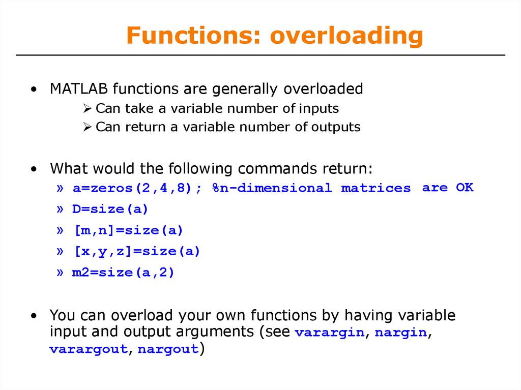
• MATLAB functions are generally overloaded
Can take a variable number of inputs
Can return a variable number of outputs
• What would the following commands return:
» a=zeros(2,4,8); %n-dimensional matrices are OK
» D=size(a)
» [m,n]=size(a)
» [x,y,z]=size(a)
» m2=size(a,2)
• You can overload your own functions by having variable
input and output arguments (see varargin, nargin,
varargout, nargout)

20. Exercise: Conditionals

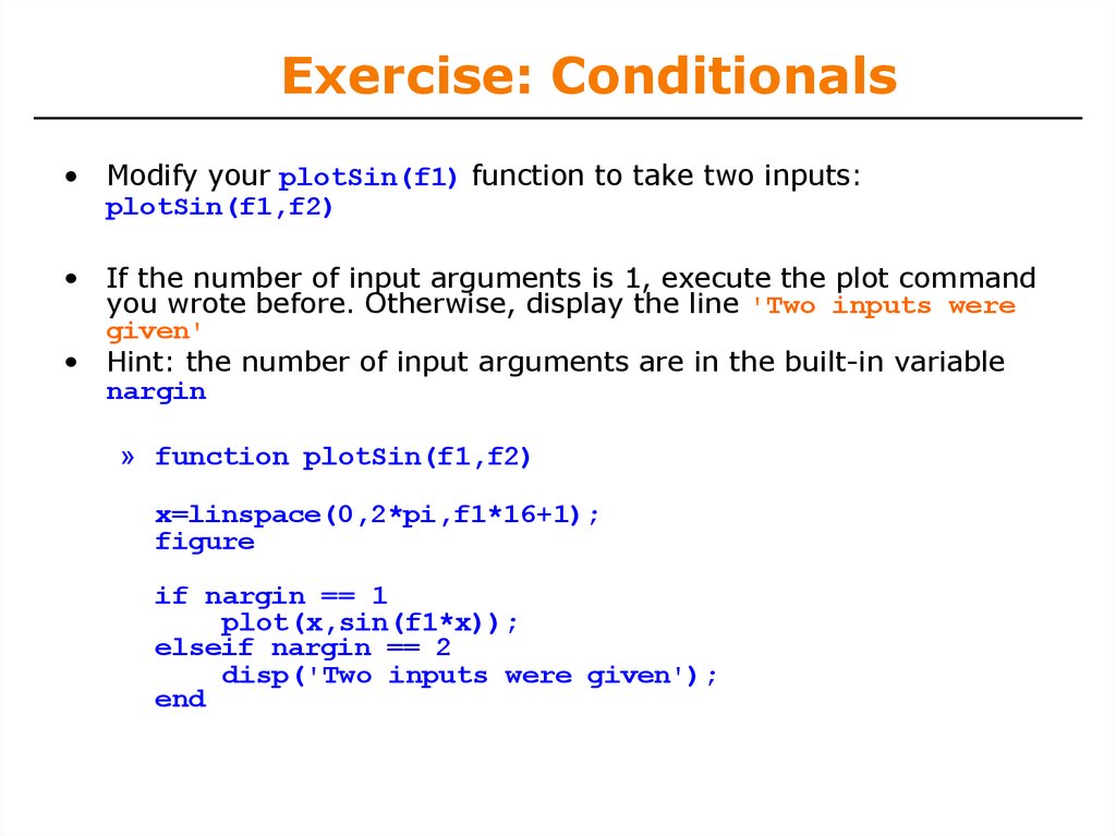
• Modify your plotSin(f1) function to take two inputs:
plotSin(f1,f2)
• If the number of input arguments is 1, execute the plot command
you wrote before. Otherwise, display the line 'Two inputs were
given'
• Hint: the number of input arguments are in the built-in variable
nargin
» function plotSin(f1,f2)
x=linspace(0,2*pi,f1*16+1);
figure
if nargin == 1
plot(x,sin(f1*x));
elseif nargin == 2
disp('Two inputs were given');
end

21. Plotting

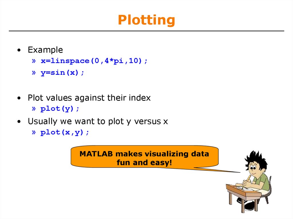
• Example
» x=linspace(0,4*pi,10);
» y=sin(x);
• Plot values against their index
» plot(y);
• Usually we want to plot y versus x
» plot(x,y);
MATLAB makes visualizing data
fun and easy!

22. What does plot do?

• plot generates dots at each (x,y) pair and then connects the dots
with a line
• To make plot of a function look smoother, evaluate at more points
» x=linspace(0,4*pi,1000);
» plot(x,sin(x));
• x and y vectors must be same size or else you’ll get an error
» plot([1 2], [1 2 3])
error!!
1
10 x values:
1
1000 x values:
0.8
0.6
0.
8
0.
6
0.4
0.
4
0.2
0.
2
0
-0.2
0
-0.4
0.2
-0.6
0.4
-0.8
-1 0
2
4
6
8
1
0
1
2
1
4
0.6
0.8
0
2
4
6
8
1
0
1
2
1
4

23. Outline

(1)
(2)
(3)
(4)
(5)
Functions
Flow Control
Line Plots
Image/Surface Plots
Vectorization

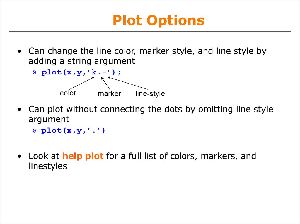
24. Plot Options

• Can change the line color, marker style, and line style by
adding a string argument
» plot(x,y,’k.-’);
color
marker
line-style
• Can plot without connecting the dots by omitting line style
argument
» plot(x,y,’.’)
• Look at help plot for a full list of colors, markers, and
linestyles

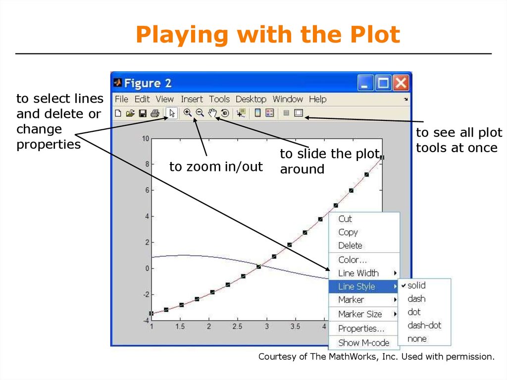
25. Playing with the Plot

to select lines
and delete or
change
properties
to zoom in/out
to slide the plot
around
to see all plot
tools at once
Courtesy of The MathWorks, Inc. Used with permission.

26. Line and Marker Options

• Everything on a line can be customized
» plot(x,y,'--s','LineWidth',2,...
'Color', [1 0 0], ...
'MarkerEdgeColor','k',...
'MarkerFaceColor','g',...
'MarkerSize',10)
You can set colors by using
a vector of [R G B] values
or a predefined color
character like 'g', 'k', etc.
0.8
0.6
0.4
0.2
0
• See doc line_props for a full list of-0.2
properties that can be specified
-0.4
-0.6
-0.8
-4
-3
-2
-1
0
1
2
3
4

27. Cartesian Plots

• We have already seen the plot function
» x=-pi:pi/100:pi;
» y=cos(4*x).*sin(10*x).*exp(-abs(x));
» plot(x,y,'k-');
• The same syntax applies for semilog and loglog plots
» semilogx(x,y,'k');
» semilogy(y,'r.-');
» loglog(x,y);
50
10
40
10
30
10
• For example:
» x=0:100;
» semilogy(x,exp(x),'k.-');
20
10
10
10
10
0
0
10
20
30
40
50
60
70
80
90
100

28. 3D Line Plots

• We can plot in 3 dimensions just as easily as in 2
» time=0:0.001:4*pi;
» x=sin(time);
» y=cos(time);
» z=time;
» plot3(x,y,z,'k','LineWidth',2);
» zlabel('Time');
10
• Use tools on figure to rotate it
• Can set limits on all 3 axes
» xlim, ylim, zlim
5
0
-5
-10
1
0.5
1
0.5
0
0
-0.5
-0.5
-1
-1

29. Axis Modes

• Built-in axis modes
» axis square
makes the current axis look like a box
» axis tight
fits axes to data
» axis equal
makes x and y scales the same
» axis xy
puts the origin in the bottom left corner (default for plots)
» axis ij
puts the origin in the top left corner (default for
matrices/images)

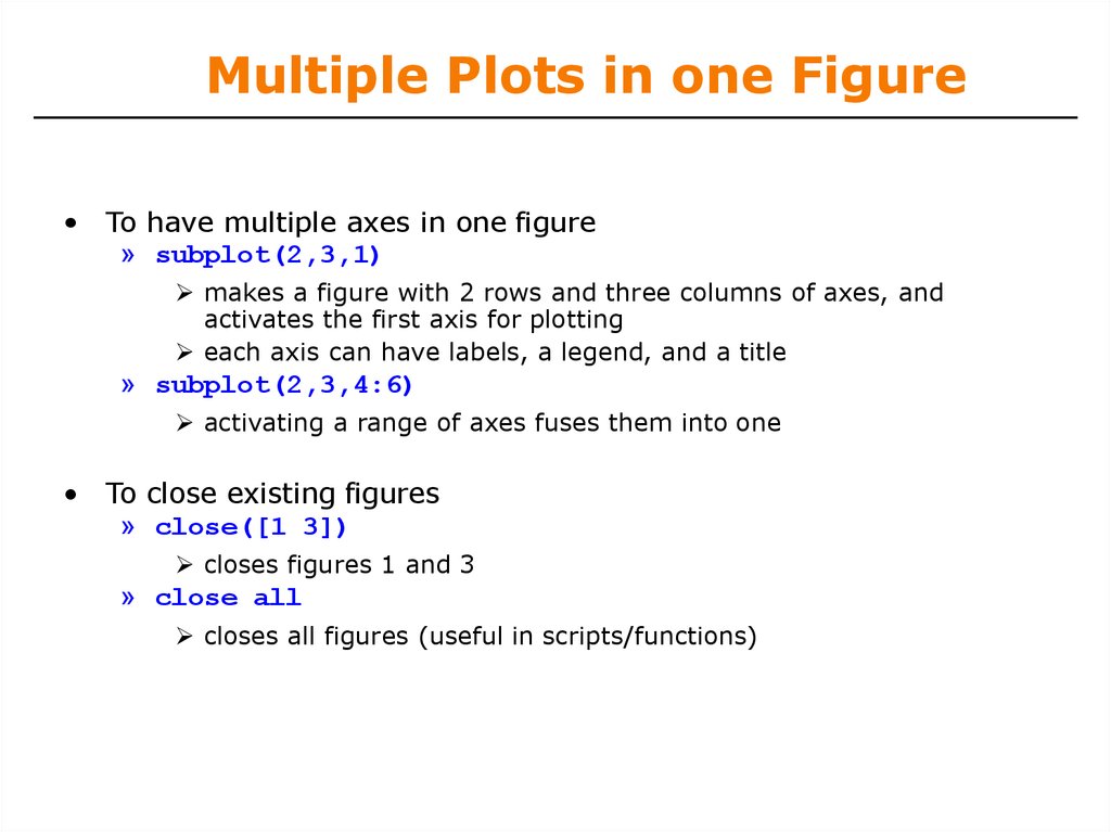
30. Multiple Plots in one Figure

• To have multiple axes in one figure
» subplot(2,3,1)
makes a figure with 2 rows and three columns of axes, and
activates the first axis for plotting
each axis can have labels, a legend, and a title
» subplot(2,3,4:6)
activating a range of axes fuses them into one
• To close existing figures
» close([1 3])
closes figures 1 and 3
» close all
closes all figures (useful in scripts/functions)

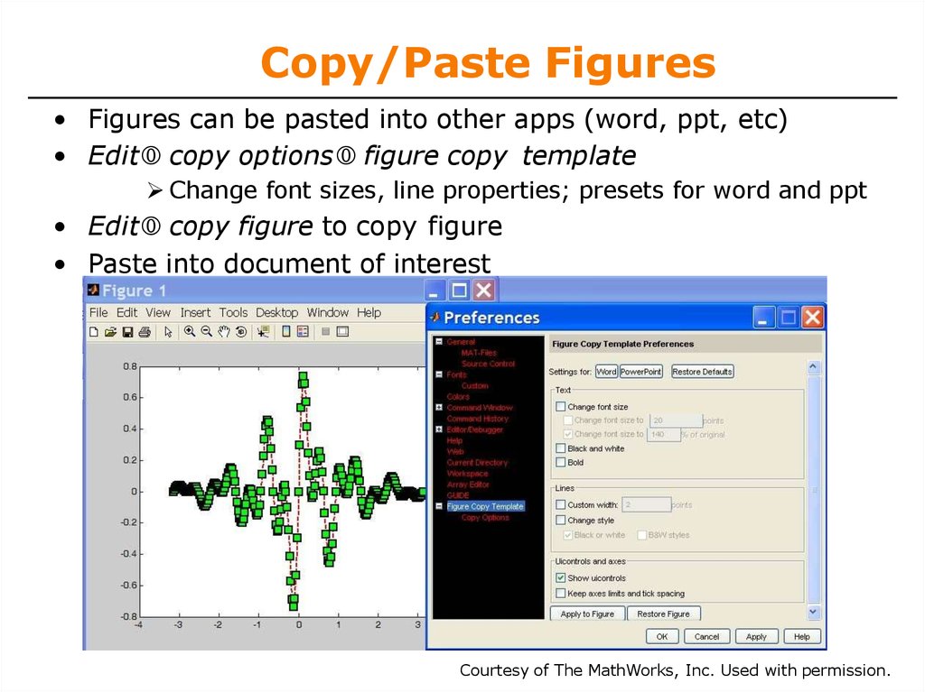
31. Copy/Paste Figures

• Figures can be pasted into other apps (word, ppt, etc)
• Edit copy options figure copy template
Change font sizes, line properties; presets for word and ppt
• Edit copy figure to copy figure
• Paste into document of interest
Courtesy of The MathWorks, Inc. Used with permission.

32. Saving Figures

• Figures can be saved in many formats. The common ones
are:
.fig preserves all
information
.bmp uncompressed
image
.eps high-quality
scaleable format
.pdf compressed
image
Courtesy of The MathWorks, Inc. Used with permission.

33. Outline

(1)
(2)
(3)
(4)
(5)
Functions
Flow Control
Line Plots
Image/Surface Plots
Vectorization

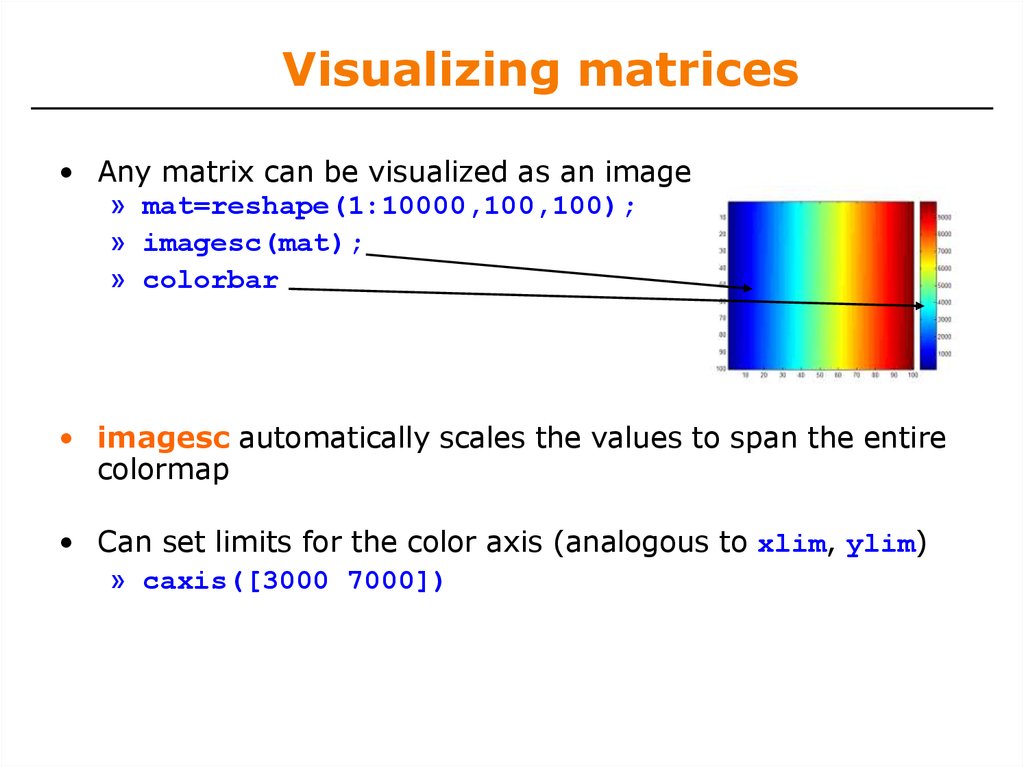
34. Visualizing matrices

• Any matrix can be visualized as an image
» mat=reshape(1:10000,100,100);
» imagesc(mat);
» colorbar
• imagesc automatically scales the values to span the entire
colormap
• Can set limits for the color axis (analogous to xlim, ylim)
» caxis([3000 7000])

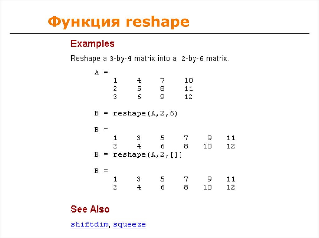
35. Функция reshape

36. Colormaps

• You can change the colormap:
» imagesc(mat)
default map is jet
» colormap(gray)
» colormap(cool)
» colormap(hot(256))
• See help hot for a list
• Can define custom colormap
» map=zeros(256,3);
» map(:,2)=(0:255)/255;
» colormap(map);

37. Surface Plots

• It is more common to visualize surfaces in 3D
• Example:
f x, y sin x cos y
x , ; y ,
• surf puts vertices at specified points in space x,y,z, and
connects all the vertices to make a surface
• The vertices can be denoted by matrices X,Y,Z
3
• How can we make these matrices
loop (DUMB)
built-in function: meshgrid
2
4
3
2
6
2
1
8
4
2
10
0
6
1
12
8
-1
14
10
0
16
12
-2
18
-1
14
20
16
-3
2
-2
18
20
-3
2
4
6
8
10
12
14
16
18
20
4
6
8
10
12
14
16
18
20

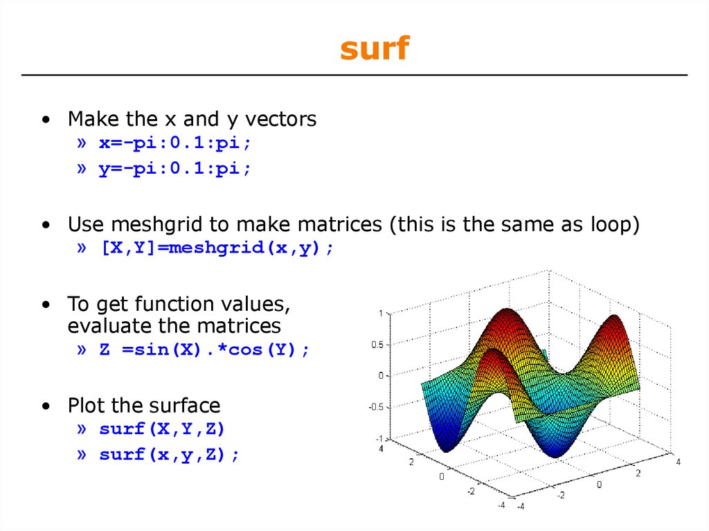
38. surf

• Make the x and y vectors
» x=-pi:0.1:pi;
» y=-pi:0.1:pi;
• Use meshgrid to make matrices (this is the same as loop)
» [X,Y]=meshgrid(x,y);
• To get function values,
evaluate the matrices
» Z =sin(X).*cos(Y);
• Plot the surface
» surf(X,Y,Z)
» surf(x,y,Z);

39. surf Options

• See help surf for more options
• There are three types of surface shading
» shading faceted
» shading flat
» shading interp
• You can change colormaps
» colormap(gray)

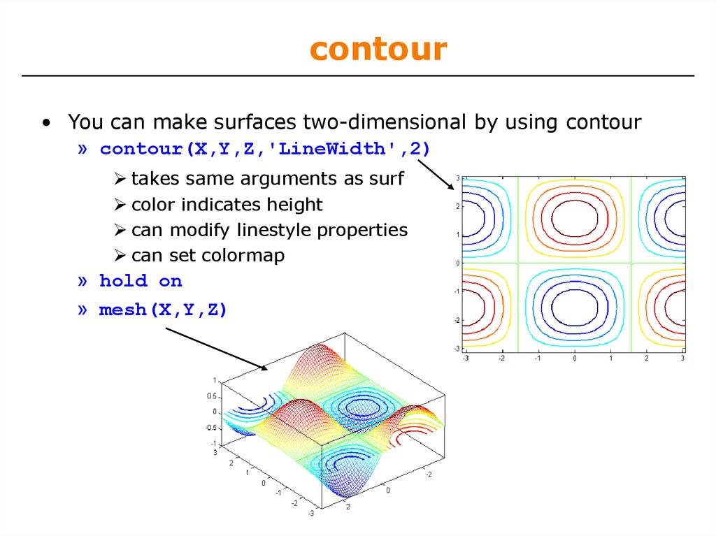
40. contour

• You can make surfaces two-dimensional by using contour
» contour(X,Y,Z,'LineWidth',2)
takes same arguments as surf
color indicates height
can modify linestyle properties
can set colormap
» hold on
» mesh(X,Y,Z)

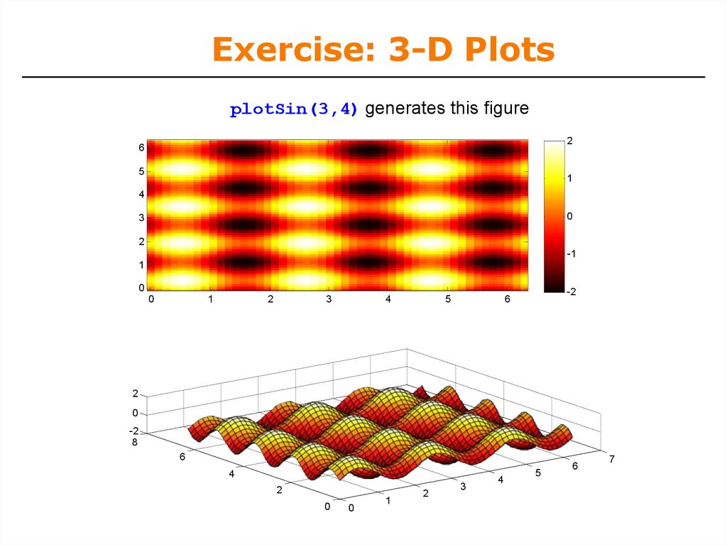
41. Exercise: 3-D Plots

• Modify plotSin to do the following:
• If two inputs are given, evaluate the following function:
Z sin f1 x sin f2 y
• y should be just like x, but using f2. (use meshgrid to get
the X and Y matrices)
• In the top axis of your subplot, display an image of the Z
matrix. Display the colorbar and use a hot colormap. Set
the axis to xy (imagesc, colormap, colorbar, axis)
• In the bottom axis of the subplot, plot the 3-D surface of Z
(surf)

42. Exercise: 3-D Plots

» function plotSin(f1,f2)
x=linspace(0,2*pi,round(16*f1)+1);
figure
if nargin == 1
plot(x,sin(f1*x),'rs--',...
'LineWidth',2,'MarkerFaceColor','k');
elseif nargin == 2
y=linspace(0,2*pi,round(16*f2)+1);
[X,Y]=meshgrid(x,y);
Z=sin(f1*X)+sin(f2*Y);
subplot(2,1,1); imagesc(x,y,Z); colorbar;
axis xy; colormap hot
subplot(2,1,2); surf(X,Y,Z);
end

43. Exercise: 3-D Plots

plotSin(3,4) generates this figure
2
6
5
1
4
0
3
2
-1
1
0
1
0
2
3
4
5
-2
6
2
0
-2
8
6
4
2
0
0
1
2
3
4
5
6
7

44. Specialized Plotting Functions

• MATLAB has a lot of specialized plotting functions
• polar-to make polar plots
» polar(0:0.01:2*pi,cos((0:0.01:2*pi)*2))
• bar-to make bar graphs
» bar(1:10,rand(1,10));
• quiver-to add velocity vectors to a plot
» [X,Y]=meshgrid(1:10,1:10);
» quiver(X,Y,rand(10),rand(10));
• stairs-plot piecewise constant functions
» stairs(1:10,rand(1,10));
• fill-draws and fills a polygon with specified vertices
» fill([0 1 0.5],[0 0 1],'r');
• see help on these functions for syntax
• doc specgraph – for a complete list