Wavelets Transform & Multiresolution Analysis

1. Wavelets Transform & Multiresolution Analysis

Wavelets Transform & Multiresolution Analysis

2. Why transform?

3.

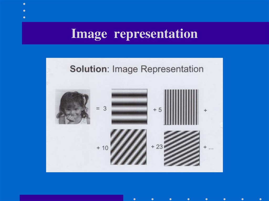
Image representation

4. Noise in Fourier spectrum

5.

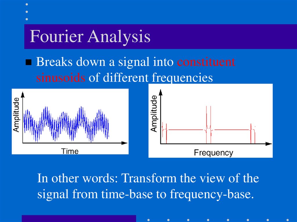
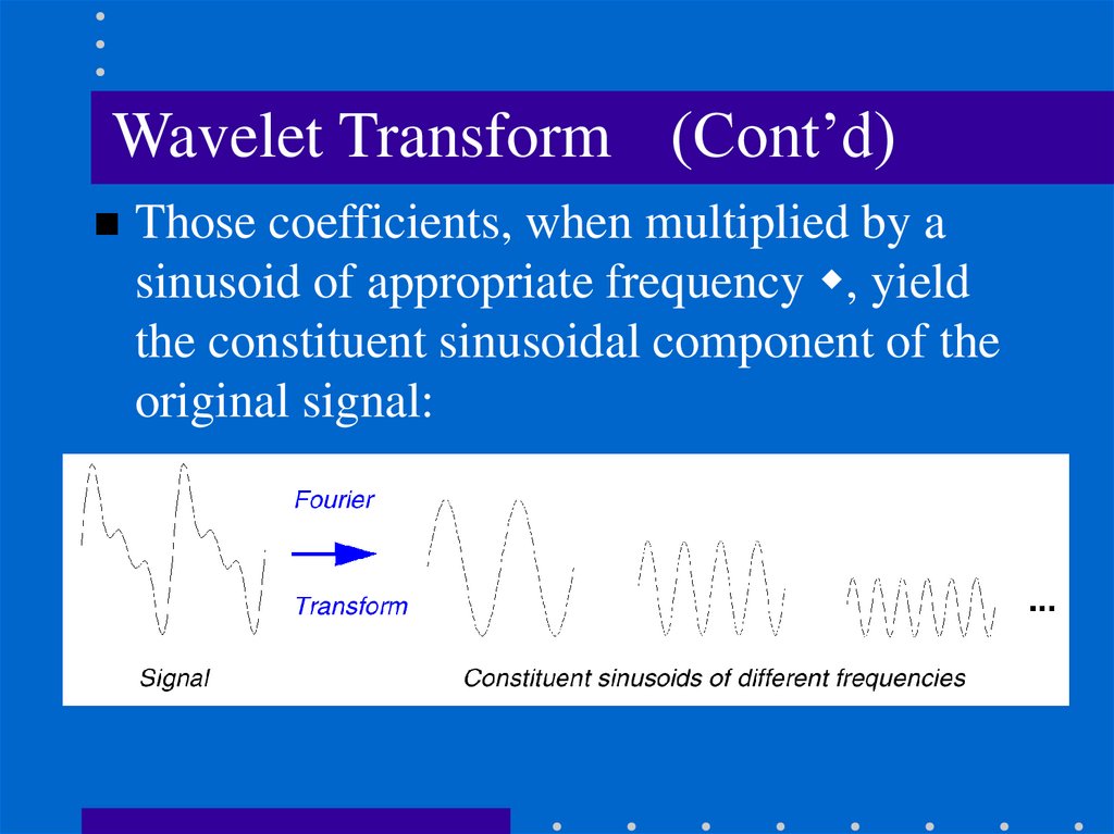
Fourier Analysis
Breaks down a signal into constituent
sinusoids of different frequencies
In other words: Transform the view of the
signal from time-base to frequency-base.

6.

What’s wrong with Fourier?
By using Fourier Transform , we loose the
time information : WHEN did a particular
event take place ?
FT can not locate drift, trends, abrupt
changes, beginning and ends of events, etc.
Calculating use complex numbers.

7. Time and Space definition

• Time – for one dimension waves we start point
shifting from source to end in time scale .
• Space – for image point shifting is two
dimensional .
• Here they are synonyms .

8.

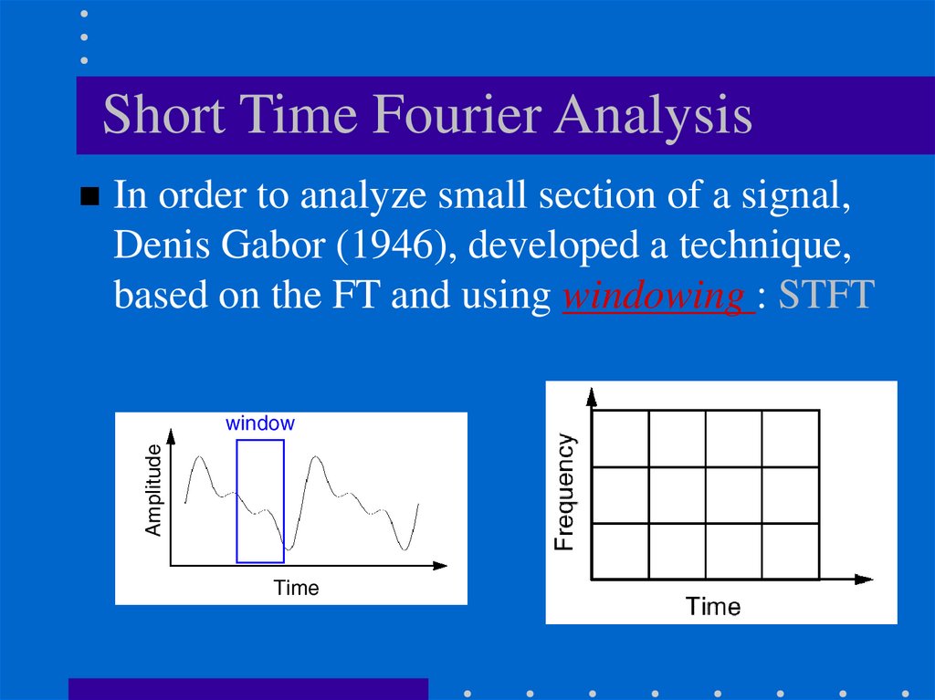
Short Time Fourier Analysis
In order to analyze small section of a signal,
Denis Gabor (1946), developed a technique,
based on the FT and using windowing : STFT

9.

STFT (or: Gabor Transform)
A compromise between time-based and
frequency-based views of a signal.
both time and frequency are represented in
limited precision.
The precision is determined by the size of
the window.
Once you choose a particular size for the
time window - it will be the same for all
frequencies.

10.

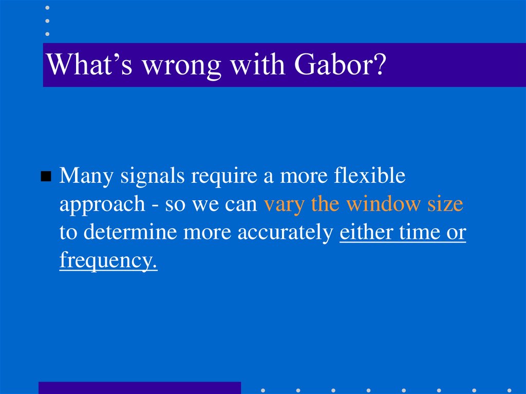
What’s wrong with Gabor?
Many signals require a more flexible
approach - so we can vary the window size
to determine more accurately either time or
frequency.

11.

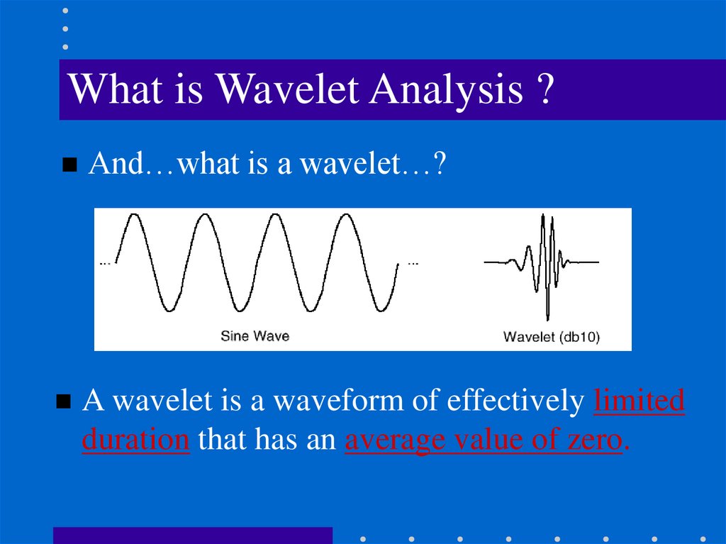
What is Wavelet Analysis ?
And…what is a wavelet…?
A wavelet is a waveform of effectively limited
duration that has an average value of zero.

12. Wavelet's properties

• Short time localized waves with zero integral value.
• Possibility of time shifting.
• Flexibility.

13.

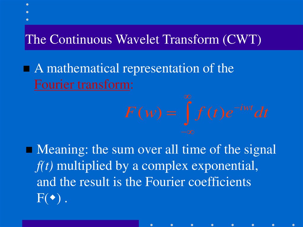
The Continuous Wavelet Transform (CWT)
A mathematical representation of the
Fourier transform:
F ( w) f (t )e
iwt
dt
Meaning: the sum over all time of the signal
f(t) multiplied by a complex exponential,
and the result is the Fourier coefficients
F( ) .

14.

Wavelet Transform (Cont’d)
Those coefficients, when multiplied by a
sinusoid of appropriate frequency , yield
the constituent sinusoidal component of the
original signal:

15.

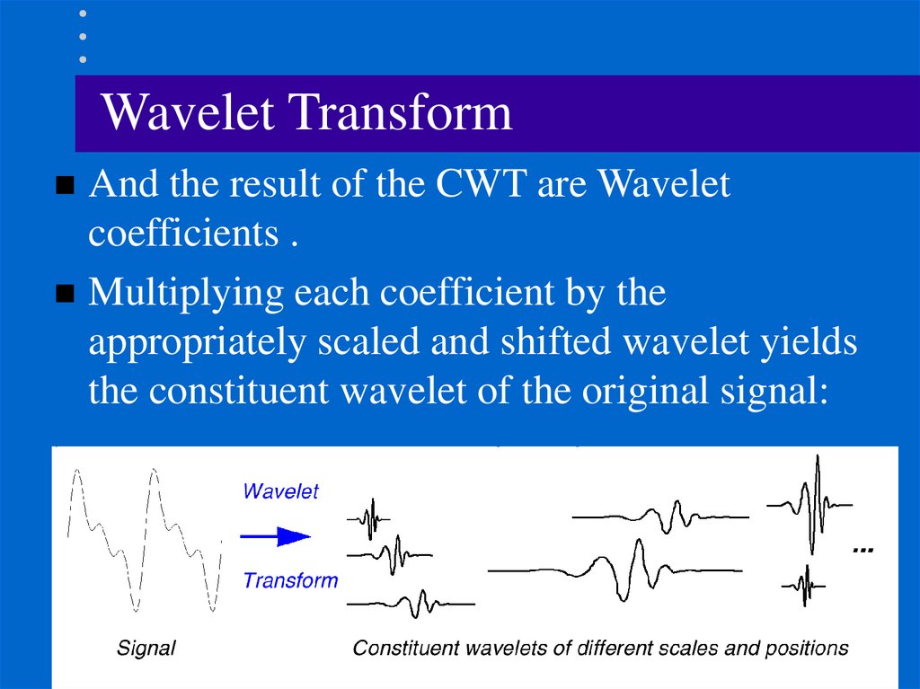
Wavelet Transform
And the result of the CWT are Wavelet
coefficients .
Multiplying each coefficient by the
appropriately scaled and shifted wavelet yields
the constituent wavelet of the original signal:

16.

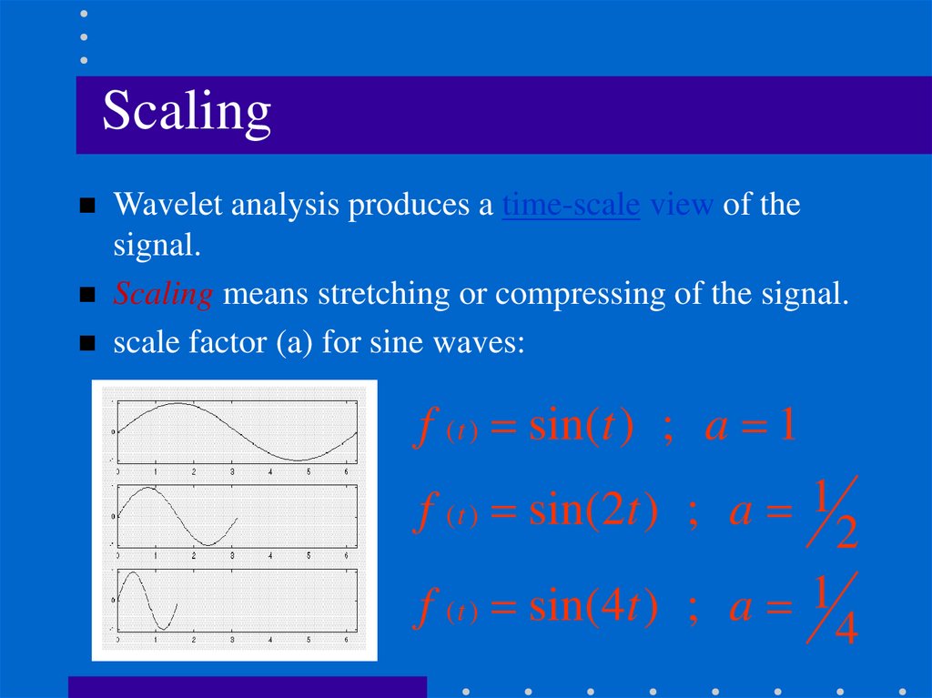
Scaling
Wavelet analysis produces a time-scale view of the
signal.
Scaling means stretching or compressing of the signal.
scale factor (a) for sine waves:
f ( t ) sin(t ) ; a 1
f ( t ) sin(2t ) ; a 1 2
f ( t ) sin(4t ) ; a 1 4

17.

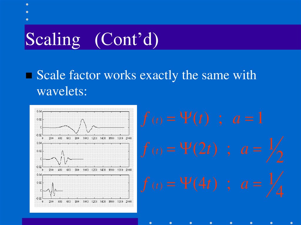
Scaling (Cont’d)
Scale factor works exactly the same with
wavelets:
f ( t ) (t ) ; a 1
f ( t ) ( 2t ) ; a 1 2
f ( t ) ( 4t ) ; a 1 4

18.

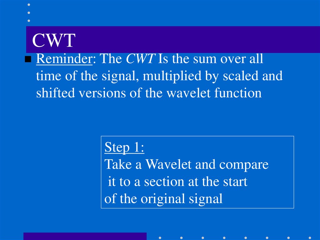
CWT
Reminder: The CWT Is the sum over all
time of the signal, multiplied by scaled and
shifted versions of the wavelet function
Step 1:
Take a Wavelet and compare
it to a section at the start
of the original signal

19.

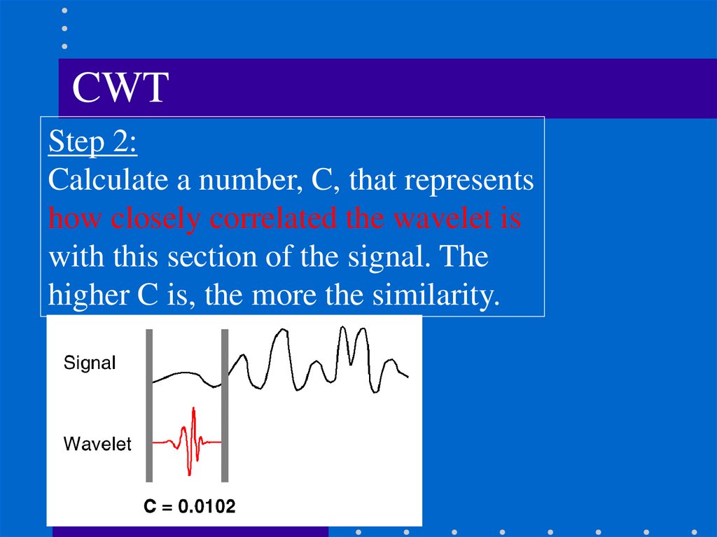
CWT
Step 2:
Calculate a number, C, that represents
how closely correlated the wavelet is
with this section of the signal. The
higher C is, the more the similarity.

20.

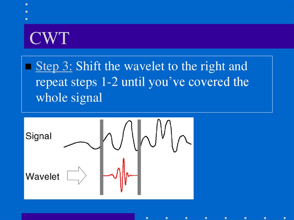
CWT
Step 3: Shift the wavelet to the right and
repeat steps 1-2 until you’ve covered the
whole signal

21.

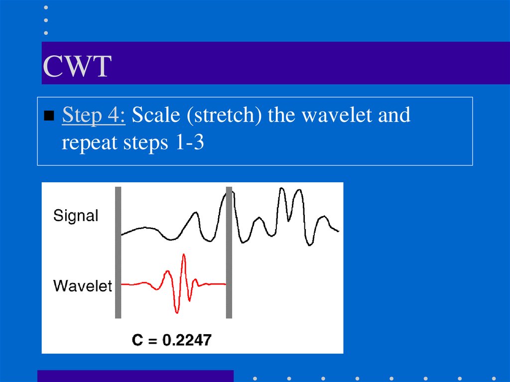
CWT
Step 4: Scale (stretch) the wavelet and
repeat steps 1-3

22. STFT - revisited

• Time - Frequency localization depends on window size.
– Wide window good frequency localization, poor time localization.
– Narrow window good time localization, poor frequency localization.

23. Wavelet Transform

• Uses a variable length window, e.g.:
– Narrower windows are more appropriate at high frequencies
– Wider windows are more appropriate at low frequencies

24. What is a wavelet?

• A function that “waves” above and below the x-axis with
the following properties:
– Varying frequency
– Limited duration
– Zero average value
• This is in contrast to sinusoids, used by FT, which have
infinite duration and constant frequency.
Sinusoid
Wavelet

25. Types of Wavelets

• There are many different wavelets, for example:
Haar
Morlet
Daubechies

26. Basis Functions Using Wavelets

• Like sin( ) and cos( ) functions in the Fourier Transform,
wavelets can define a set of basis functions ψk(t):
f (t ) ak k (t )
k
• Span of ψk(t): vector space S containing all functions f(t)
that can be represented by ψk(t).

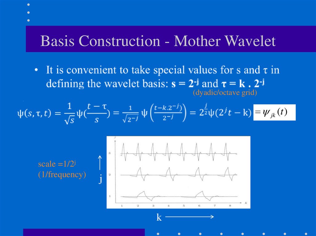
27.

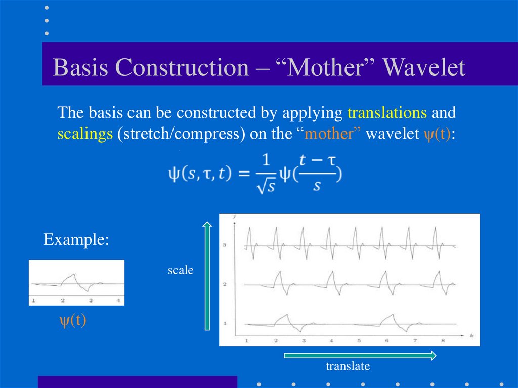
Basis Construction – “Mother” Wavelet
The basis can be constructed by applying translations and
scalings (stretch/compress) on the “mother” wavelet ψ(t):
Example:
scale
ψ(t)
translate

28.

Basis Construction - Mother Wavelet
(dyadic/octave grid)
jk (t )
scale =1/2j
(1/frequency)
j
k

29. Continuous Wavelet Transform (CWT)

translation parameter
(measure of time)
Forward
CWT:
scale parameter
(measure of frequency)
scale =1/2j
(1/frequency)
1
t
C ( , s)
f t
dt
s t
s
normalization
constant
mother wavelet (i.e.,
window function)

30. Illustrating CWT

1. Take a wavelet and compare it to a section at the start
of the original signal.
2. Calculate a number, C, that represents how closely
correlated the wavelet is with this section of the
signal. The higher C is, the more the similarity.
C ( , s)
1
t
f
t
dt
s t
s

31. Illustrating CWT (cont’d)

3. Shift the wavelet to the right and repeat step 2 until you've
covered the whole signal.
C ( , s)
1
t
f t
dt
s t
s

32. Illustrating CWT (cont’d)

4. Scale the wavelet and go to step 1.
C ( , s)
1
t
f t
dt
s t
s
5. Repeat steps 1 through 4 for all scales.

33. Visualize CTW Transform

• Wavelet analysis produces a time-scale view of the input
signal or image.
C ( , s)
1
t
f t
dt
s t
s

34. Continuous Wavelet Transform (cont’d)

1
t
f t
Forward CWT: C ( , s)
dt
s t
s
Inverse CWT:
1
t
f (t )
C ( , s) (
)d ds
s
s s
Note the double integral!

35. Fourier Transform vs Wavelet Transform

weighted by F(u)

36. Fourier Transform vs Wavelet Transform

weighted by C(τ,s)
1
t
f (t )
C ( , s) (
)d ds
s
s s

37. Properties of Wavelets

• Simultaneous localization in time and scale
- The location of the wavelet allows to explicitly represent
the location of events in time.
- The shape of the wavelet allows to represent different
detail or resolution.

38. Properties of Wavelets (cont’d)

• Sparsity: for functions typically found in practice, many
of the coefficients in a wavelet representation are either
zero or very small.
1
t
f (t )
C ( , s) (
)d ds
s
s s

39. Properties of Wavelets (cont’d)

1
t
f (t )
C ( , s) (
)d ds
s
s s
• Adaptability: Can represent functions with discontinuities
or corners more efficiently.
• Linear-time complexity: many wavelet transformations
can be accomplished in O(N) time.

40. Discrete Wavelet Transform (DWT)

a jk f (t ) *jk (t )
(forward DWT)
t
f (t ) a jk jk (t )
k
where
j
(inverse DWT)
jk (t ) 2 j / 2 2 j t k

41. DFT vs DWT

• DFT expansion:
one parameter basis
or
f (t ) a l l (t )
l
• DWT expansion two parameter basis
f (t ) a jk jk (t )
k
j

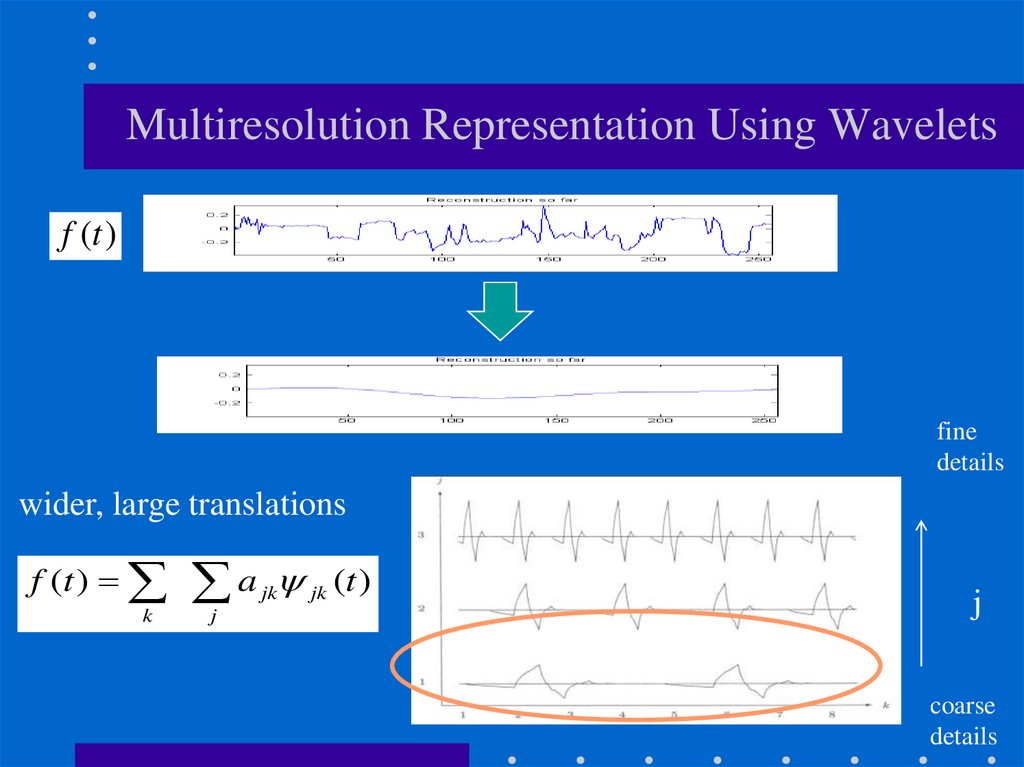
42.

Multiresolution Representation Using Wavelets
f (t )
fine
details
wider, large translations
f (t ) a jk jk (t )
k
j
j
coarse
details

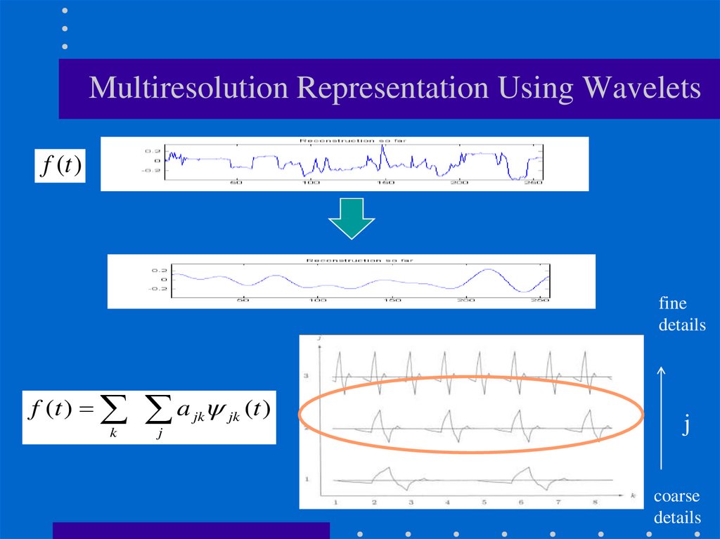
43.

Multiresolution Representation Using Wavelets
f (t )
fine
details
f (t ) a jk jk (t )
k
j
j
coarse
details

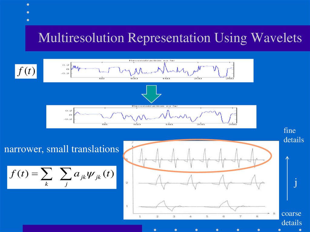
44.

Multiresolution Representation Using Wavelets
f (t )
fine
details
narrower, small translations
f (t ) a jk jk (t )
k
j
j
coarse
details

45.

Multiresolution Representation Using Wavelets
high resolution
f (t )
(more details)
fˆ1 (t )
fˆ2 (t )
j
…
low resolution
fˆs (t )
(less details)
f (t ) a jk jk (t )
k
j

46.

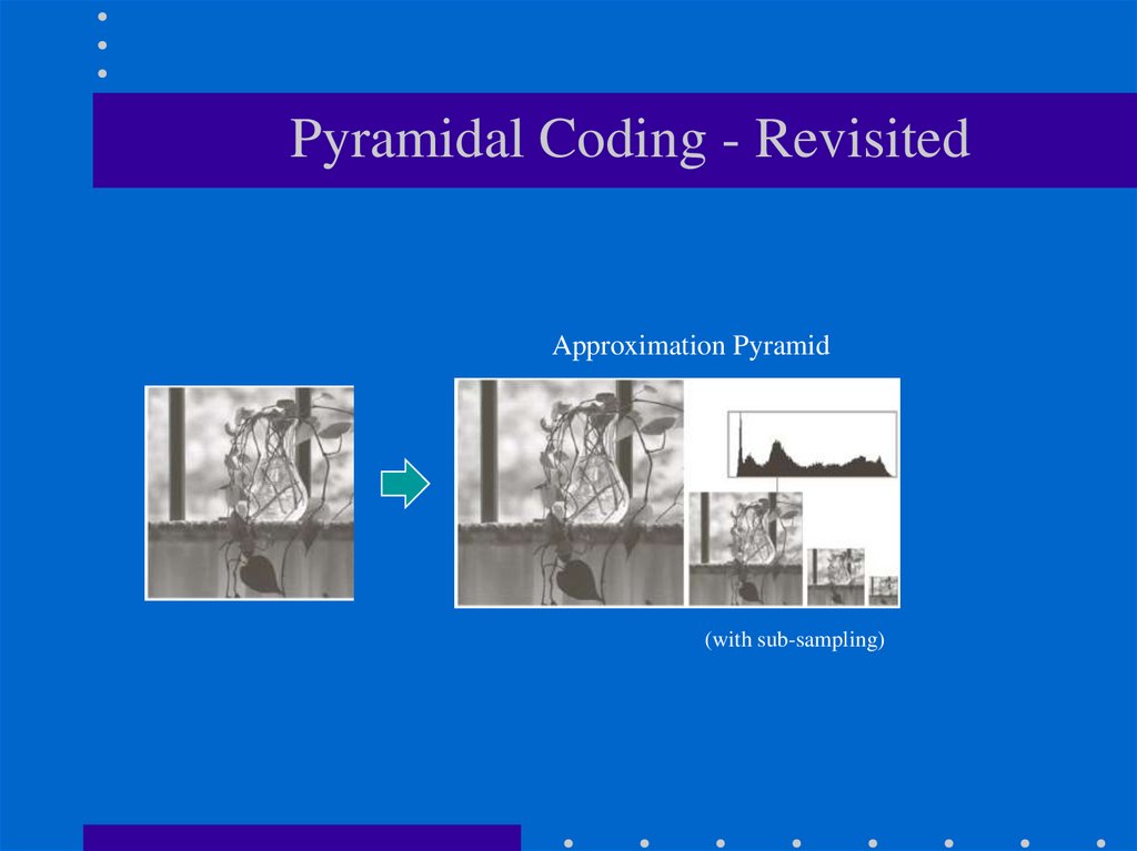
Pyramidal Coding - Revisited
Approximation Pyramid
(with sub-sampling)

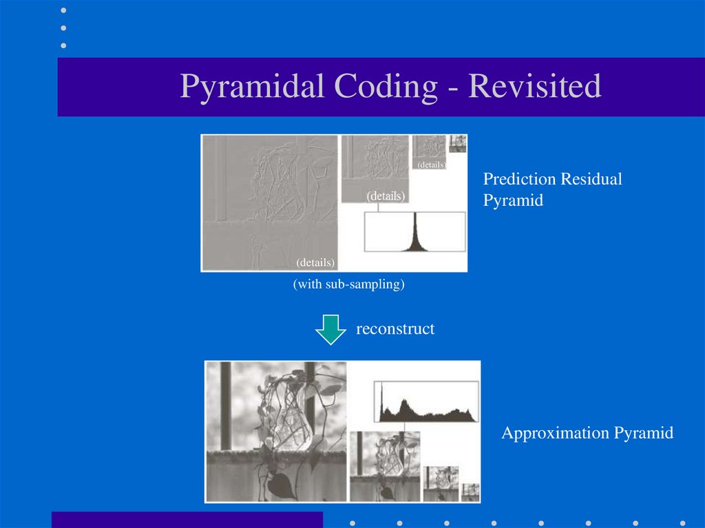
47.

Pyramidal Coding - Revisited
(details)
Prediction Residual
Pyramid
(details)
(with sub-sampling)
reconstruct
Approximation Pyramid

48.

Efficient Representation Using “Details”
details D3
details D2
details D1
L0
(without sub-sampling)

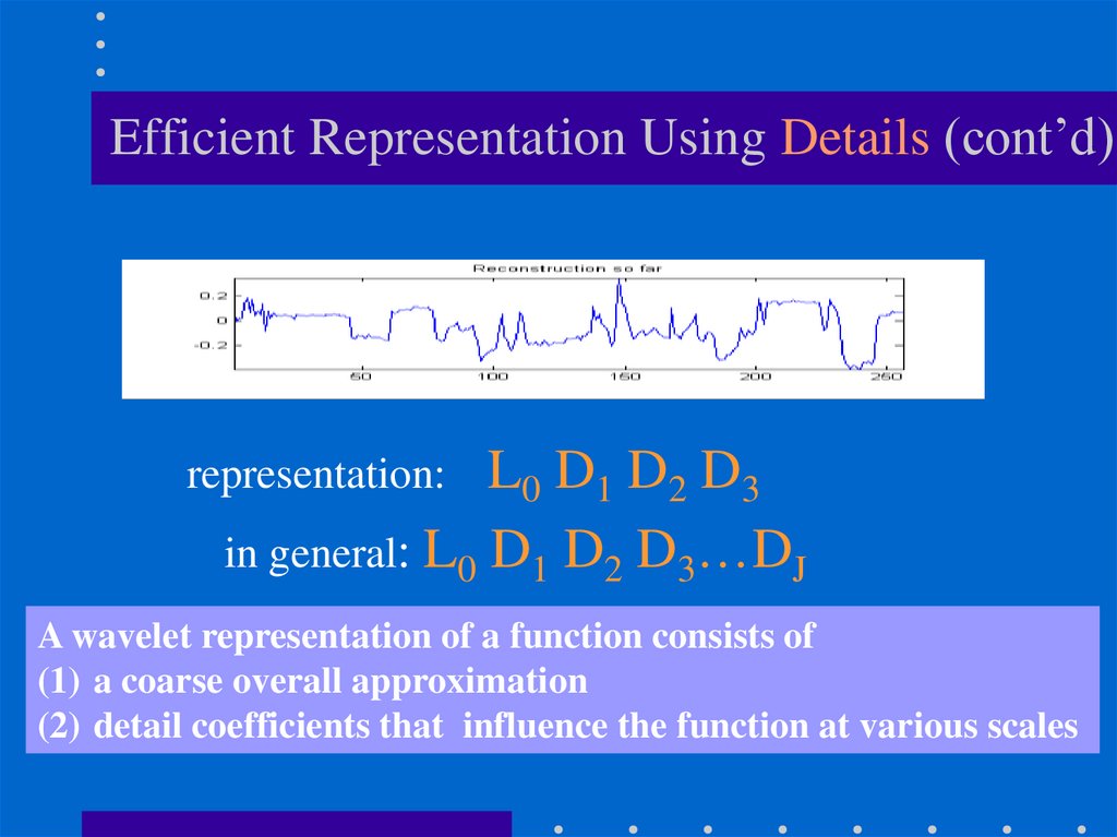
49.

Efficient Representation Using Details (cont’d)
L0 D1 D2 D3
in general: L0 D1 D2 D3…DJ
representation:
A wavelet representation of a function consists of
(1) a coarse overall approximation
(2) detail coefficients that influence the function at various scales

50. Reconstruction (synthesis)

H3=H2 & D3
details D3
H2=H1 & D2
details D2
H1=L0 & D1
details D1
L0
(without sub-sampling)

51. Example - Haar Wavelets

• Suppose we are given a 1D "image" with a resolution
of 4 pixels:
[9 7 3 5]
• The Haar wavelet transform is the following:
(with sub-sampling)
L0 D1 D2 D3

52. Example - Haar Wavelets (cont’d)

• Start by averaging and subsampling the pixels
together (pairwise) to get a new lower resolution
image:
[9 7 3 5]
• To recover the original four pixels from the two
averaged pixels, store some detail coefficients.
1

53. Example - Haar Wavelets (cont’d)

• Repeating this process on the averages (i.e., low
resolution image) gives the full decomposition:
1
Harr decomposition:

54. Example - Haar Wavelets (cont’d)

• The original image can be reconstructed by adding or
subtracting the detail coefficients from the lowerresolution representations.
L0 D1 D2 D3
2
[6]
1 -1

55. Example - Haar Wavelets (cont’d)

Detail coefficients
become smaller and
smaller scale decreases.
Dj
Dj-1
L0
D1
How should we
compute the detail
coefficients Dj ?

56. Multiresolution Conditions

• If a set of functions V can be represented by a weighted
sum of ψ(2jt - k), then a larger set, including V, can be
represented by a weighted sum of ψ(2j+1t - k).
high
resolution
ψ(2j+1t - k)
j
ψ(2jt - k)
low
resolution

57. Multiresolution Conditions (cont’d)

Vj+1: span of ψ(2j+1t - k):
Vj: span of ψ(2jt - k):
f j 1 (t ) bk ( j 1) k (t )
k
f j (t ) ak jk (t )
k
V j V j 1

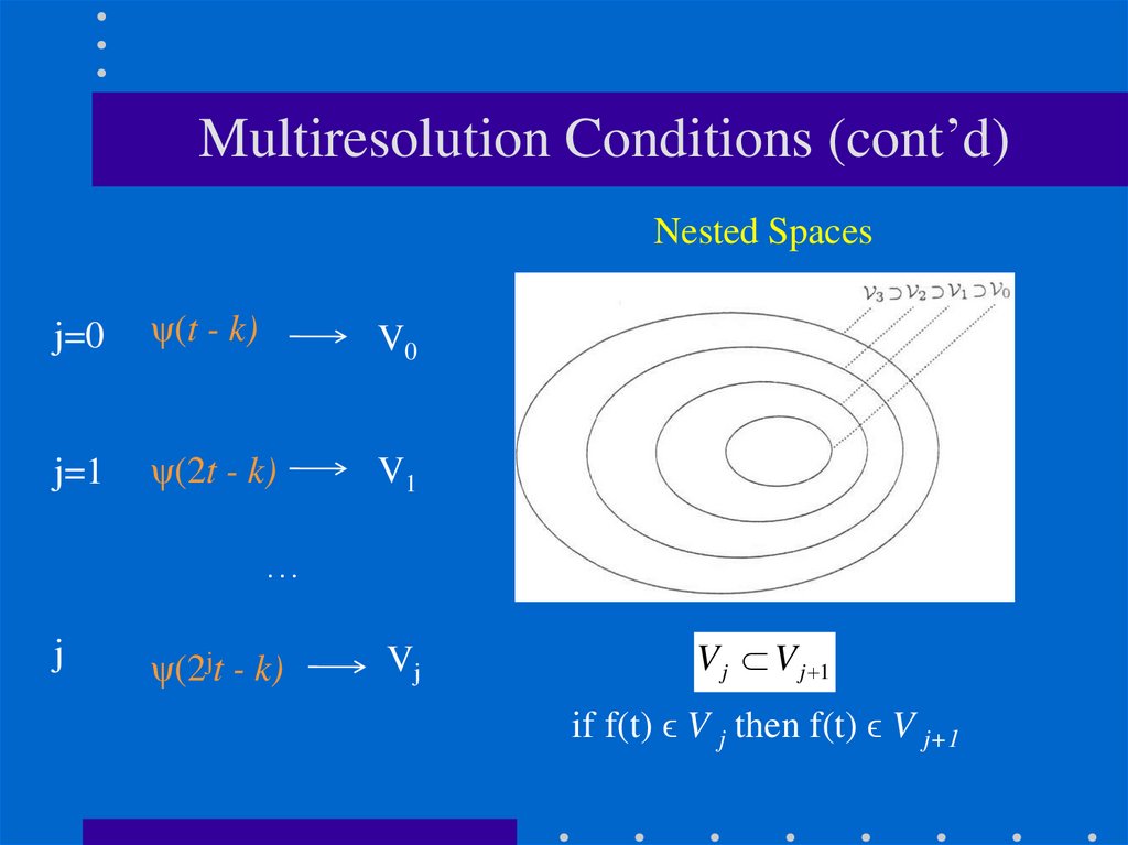
58.

Multiresolution Conditions (cont’d)
Nested Spaces
j=0
ψ(t - k)
V0
j=1
ψ(2t - k)
V1
…
j
ψ(2jt - k)
Vj
V j V j 1
if f(t) ϵ V j then f(t) ϵ V j+1

59. How to compute Dj ?

IDEA:
Define a set of basis functions
that span the difference
between Vj+1 and Vj

60.

How to compute Dj ? (cont’d)
• Let Wj be the orthogonal complement of Vj in Vj+1
Vj+1 = Vj + Wj

61.

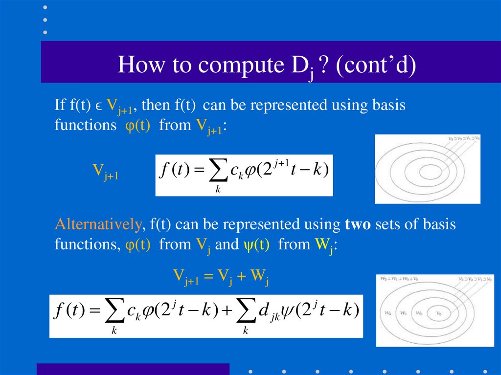
How to compute Dj ? (cont’d)
If f(t) ϵ Vj+1, then f(t) can be represented using basis
functions φ(t) from Vj+1:
Vj+1
f (t ) ck (2 j 1 t k )
k
Alternatively, f(t) can be represented using two sets of basis
functions, φ(t) from Vj and ψ(t) from Wj:
Vj+1 = Vj + Wj
f (t ) ck (2 j t k ) d jk (2 j t k )
k
k

62.

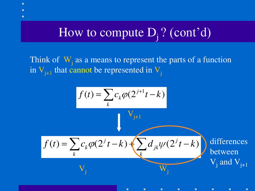
How to compute Dj ? (cont’d)
Think of Wj as a means to represent the parts of a function
in Vj+1 that cannot be represented in Vj
f (t ) ck (2 j 1 t k )
k
Vj+1
f (t ) ck (2 j t k ) d jk (2 j t k )
k
k
Vj
Wj
differences
between
Vj and Vj+1

63.

How to compute Dj ? (cont’d)
Vj+1 = Vj + Wj using recursion on Vj:
Vj+1 = Vj-1+Wj-1+Wj = …= V0 + W0 + W1 + W2 + … + Wj
if f(t) ϵ Vj+1 , then:
f (t ) ck (t k ) d jk (2 j t k )
k
k
j
V0
W0, W1, W2, …
basis functions
basis functions

64. Summary: wavelet expansion (Section 7.2)

• Wavelet decompositions involve a pair of waveforms:
encodes low
resolution info
φ(t)
ψ(t)
encodes details or
high resolution info
f (t ) ck (t k ) d jk (2 j t k )
k
Terminology:
scaling function
k
j
wavelet function

65. 1D Haar Wavelets

• Haar scaling and wavelet functions:
φ(t)
ψ(t)
computes average
(low pass)
computes details
(high pass)

66.

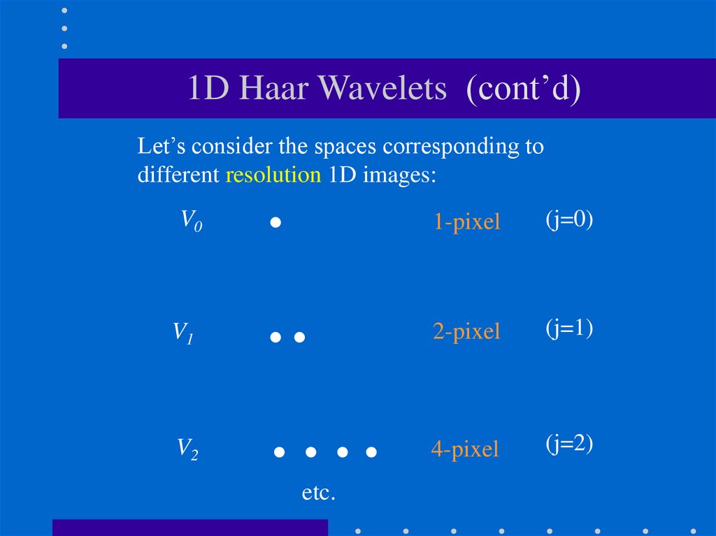
1D Haar Wavelets (cont’d)
Let’s consider the spaces corresponding to
different resolution 1D images:
V0
V1
V2
.
..
….
etc.
1-pixel
(j=0)
2-pixel
(j=1)
4-pixel
(j=2)

67. 1D Haar Wavelets (cont’d)

j=0
• V0 represents the space of 1-pixel (20-pixel) images
• Think of a 1-pixel image as a function that is constant
over [0,1)
Example:
width: 1
0
1

68. 1D Haar Wavelets (cont’d)

j=1
• V1 represents the space of all 2-pixel (21-pixel) images
• Think of a 2-pixel image as a function having 21 equalsized constant pieces over the interval [0, 1).
Example:
0
½
1
width: 1/2
Note that: V0 V1
e.g.,
=
+

69. 1D Haar Wavelets (cont’d)

• V j represents all the 2j-pixel images
• Functions having 2j equal-sized constant pieces over
interval [0,1).
Example:
width: 1/2j
Note that:
Vj-1
ϵ Vj
width: 1/2j-1
ϵ Vj
V1
width: 1/2

70. 1D Haar Wavelets (cont’d)

V0, V1, ..., Vj are nested
i.e.,
V j V j 1
Vj fine details
…
V1
V0 coarse info

71. Define a basis for Vj

• Scaling function:
• Let’s define a basis for V j :
Note new notation: i ( x) ji ( x)
j

72. Define a basis for Vj (cont’d)

width: 1/20
width: 1/2
width: 1/22
width: 1/23

73. Define a basis for Wj

• Wavelet function:
• Let’s define a basis ψ ji for Wj :
Note new notation: i ( x) ji ( x)
j

74. Define basis for Wj (cont’d)

Note
that the dot
product
between basis
functions in Vj
and Wj is zero!

75. Basis for Vj+1

Basis functions ψ ji of W j
Basis functions φ ji of V j
form a basis in V j+1

76. Define a basis for Wj (cont’d)

V3 = V2 + W2

77. Define a basis for Wj (cont’d)

V2 = V1 + W1

78. Define a basis for Wj (cont’d)

V1 = V0 + W0

79. Example - Revisited

f(x)=
V2

80. Example (cont’d)

f(x)=
φ2,0(x)
V2
φ2,1(x)
φ2,2(x)
φ2,3(x)

81. Example (cont’d)

(divide by 2 for normalization)
φ1,0(x)
V1 and W1
V2=V1+W1
φ1,1(x)
ψ1,0(x)
ψ1,1(x)

82. Example (cont’d)

83. Example (cont’d)

(divide by 2 for normalization)
V0 ,W0 and W1
V2=V1+W1=V0+W0+W1
φ0,0(x)
ψ0,0(x)
ψ1,0 (x)
ψ1,1(x)

84. Example

85. Example (cont’d)

86. Filter banks

• The lower resolution coefficients can be calculated
from the higher resolution coefficients by a treestructured algorithm (i.e., filter bank).
Subband
encoding
(analysis)
h0(-n) is a lowpass filter and h1(-n) is a highpass filter

87. Example (revisited)

[9 7 3 5]
low-pass,
down-sampling
(9+7)/2 (3+5)/2
high-pass,
down-sampling
(9-7)/2 (3-5)/2
LP
HP

88. Filter banks (cont’d)

Next level:
h0(-n) is a lowpass filter and h1(-n) is a highpass filter

89. Example (revisited)

[9 7 3 5]
low-pass,
down-sampling
high-pass,
down-sampling
LP
(8+4)/2
(8-4)/2
HP

90. Convention for illustrating 1D Haar wavelet decomposition

x
x
x
x
x
x
… x
x
…
detail
(HP)
…
re-arrange:
average
(LP)
…
…
re-arrange:
LP
…
HP

91. Examples of lowpass/highpass (analysis) filters

h0
Haar
h1
h0
Daubechies
h1

92. Filter banks (cont’d)

• The higher resolution coefficients can be calculated
from the lower resolution coefficients using a similar
structure.
Subband
encoding
(synthesis)
g0(n) is a lowpass filter and g1(n) is a highpass filter

93. Filter banks (cont’d)

Next level:
g0(n) is a lowpass filter and g1(n) is a highpass filter

94. Examples of lowpass/highpass (synthesis) filters

Haar (same as
for analysis):
g0
g1
g0
Daubechies:
+
g1

95. 2D Haar Wavelet Transform

• The 2D Haar wavelet decomposition can be computed
using 1D Haar wavelet decompositions.
– i.e., 2D Haar wavelet basis is separable
• We’ll discuss two different decompositions (i.e.,
correspond to different basis functions):
– Standard decomposition
– Non-standard decomposition

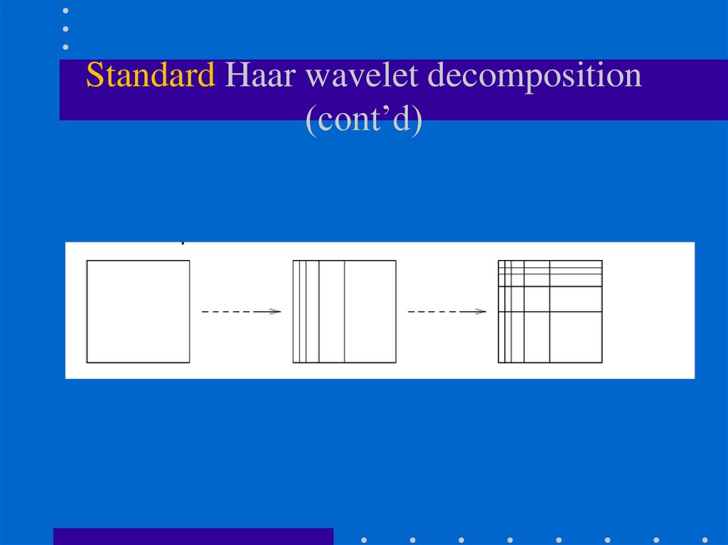
96. Standard Haar wavelet decomposition

• Steps:
(1) Compute 1D Haar wavelet decomposition of
each row of the original pixel values.
(2) Compute 1D Haar wavelet decomposition of
each column of the row-transformed pixels.

97. Standard Haar wavelet decomposition (cont’d)

average
detail
(1) row-wise Haar decomposition:
re-arrange terms
xxx
xxx
…
…
x
x
…
xxx
…
...
.
x
…
…
…
…
…
…
.
…
…
.

98. Standard Haar wavelet decomposition (cont’d)

average
detail
(1) row-wise Haar decomposition:
row-transformed result
…
…
…
…
…
.
…
…
…
…
.

99. Standard Haar wavelet decomposition (cont’d)

average
detail
(2) column-wise Haar decomposition:
row-transformed result
column-transformed result
…
…
…
…
…
…
…
.
…
…
…
…
.

100. Example

row-transformed result
…
…
re-arrange terms
…
…
…
…
.
…
…
.

101. Example (cont’d)

column-transformed result
…
…
…
…
…
.

102.

Standard Haar wavelet decomposition
(cont’d)

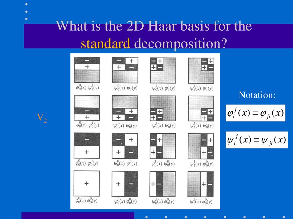
103. What is the 2D Haar basis for the standard decomposition?

To construct the standard 2D Haar wavelet basis, consider
all possible outer products of the1D basis functions.
φ0,0(x)
Example:
V2=V0+W0+W1
ψ0,0(x)
ψ1,0(x)
ψ1,1(x)

104.

What is the 2D Haar basis for the
standard decomposition?
To construct the standard 2D Haar wavelet basis, consider
all possible outer products of the1D basis functions.
φ00(x), φ00(x)
ψ00(x), φ00(x)
ψ10(x), φ00(x)
Notation: i j ( x) ji ( x) i j ( x) ji ( x)

105.

What is the 2D Haar basis for the
standard decomposition?
Notation:
V2
i j ( x) ji ( x)
i j ( x) ji ( x)

106. Non-standard Haar wavelet decomposition

• Alternates between operations on rows and columns.
(1) Perform one level decomposition in each row (i.e., one
step of horizontal pairwise averaging and differencing).
(2) Perform one level decomposition in each column from
step 1 (i.e., one step of vertical pairwise averaging and
differencing).
(3) Rearrange terms and repeat the process on the quadrant
containing the averages only.

107. Non-standard Haar wavelet decomposition (cont’d)

one level, horizontal
Haar decomposition:
xxx
xxx
…
…
x
x
…
xxx
…
...
.
x
…
one level, vertical
Haar decomposition:
…
…
…
…
…
…
.
…
…
…
.

108. Non-standard Haar wavelet decomposition (cont’d)

re-arrange terms
…
…
…
…
…
…
.
one level, horizontal
Haar decomposition
on “green” quadrant
one level, vertical
Haar decomposition
on “green” quadrant
…
…
…
…
…
…
.

109. Example

re-arrange terms
…
…
…
…
…
…
.

110. Example (cont’d)

…
…
…
…
…
.

111.

Non-standard Haar wavelet decomposition
(cont’d)

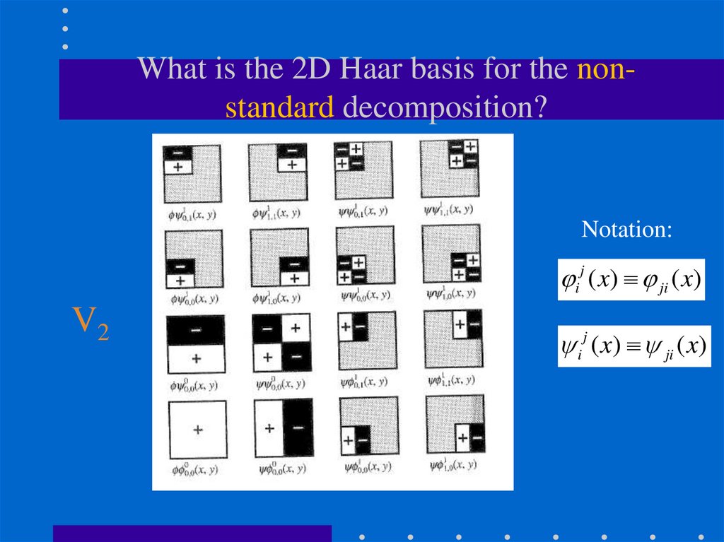
112. What is the 2D Haar basis for the non-standard decomposition?

What is the 2D Haar basis for the nonstandard decomposition?
Define 2D scaling and
wavelet functions:
Apply translations
and scaling:
( x, y) ( x) ( y)
000 ( x, y ) ( x, y )
( x, y) ( x) ( y)
( x, y) ( x) ( y)
( x, y) ( x) ( y)
kfj ( x, y ) 2 j (2 j x k , 2 j y f )
kfj ( x, y ) 2 j (2 j x k , 2 j y f )
kfj ( x, y ) 2 j (2 j x k , 2 j y f )

113.

What is the 2D Haar basis for the nonstandard decomposition?
Notation:
i j ( x) ji ( x)
V2
i j ( x) ji ( x)

114.

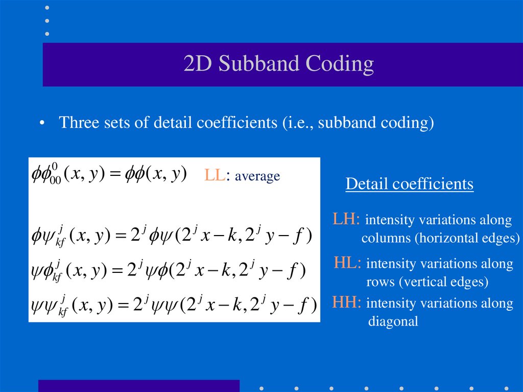
2D Subband Coding
• Three sets of detail coefficients (i.e., subband coding)
000 ( x, y ) ( x, y ) LL: average LL
Detail coefficients
( x, y ) 2 (2 x k , 2 y f )
LH: intensity variations along
kfj ( x, y ) 2 j (2 j x k , 2 j y f )
HL: intensity variations along
j
kf
j
j
j
kfj ( x, y ) 2 j (2 j x k , 2 j y f )
columns (horizontal edges)
rows (vertical edges)
HH: intensity variations along
diagonal

115. 2D Subband Coding

LL
LH
HL
HH

116. Wavelets Applications

• Noise filtering
• Image compression
– Special case: fingerprint compression
• Image fusion
• Recognition
G. Bebis, A. Gyaourova, S. Singh, and I. Pavlidis, "Face Recognition by
Fusing Thermal Infrared and Visible Imagery", Image and Vision
Computing, vol. 24, no. 7, pp. 727-742, 2006.
• Image matching and retrieval
Charles E. Jacobs Adam Finkelstein David H. Salesin, "Fast
Multiresolution Image Querying", SIGRAPH, 1995.