Similar presentations:
International Economic
1. International Economics
Seventh Edition, Global EditionChapter 4
Comparative
Advantage and
Factor
Endowments
Copyright © 2018 Pearson Education, Ltd. All Rights Reserved.
2. Learning Objectives (1 of 2)
4.1 Use the Heckscher-Ohlin Trade Model toanalyze trade patterns between two countries
with two inputs and two outputs.
4.2 Predict the impacts on different factors of
production of trade opening.
4.3 Discuss the limits of the HO model.
Copyright © 2018 Pearson Education, Ltd. All Rights Reserved.
3. Learning Objectives (2 of 2)
4.4 Explain the trade-offs for firms betweentrading and investing internationally.
4.5 Give examples of the determinants of
international migration ad its impact on
comparative advantage.
4.6 Describe the controversies surrounding the
impact of international trade on wages and jobs.
Copyright © 2018 Pearson Education, Ltd. All Rights Reserved.
4. The Heckscher-Ohlin Trade Model (1 of 6)
• Eli Heckscher and Bertil Ohlin: 20th centurySwedish economists.
– Best known for their model explaining patterns of
international trade.
– Also called the factor proportions model.
• HO Model idea: The relative abundance of
different factors of production (inputs) determine
which country has a comparative advantage in
which goods.
Copyright © 2018 Pearson Education, Ltd. All Rights Reserved.
5. The Heckscher-Ohlin Trade Model (2 of 6)
• The HO Model: 2x2x2– 2 inputs, called labor and capital.
– 2 outputs, called bread and steel.
– 2 countries, called the U.S. and Canada.
• Relative factor endowments are the ratios of
capital to labor.
– Written: K/L
Copyright © 2018 Pearson Education, Ltd. All Rights Reserved.
6. The Heckscher-Ohlin Trade Model (3 of 6)
BlankUnited States
Canada
Capital
50 machines
2 machines
Labor
150 workers
10 workers
• Factor abundance depends on the ratios of K to L.
– KCA / LCA = 2 / 10 = 1/5.
– KUS / LUS = 50 / 150 = 1/3.
• Since KUS / LUS > KCA / LCA the US is capital abundant
compared to Canada and Canada is labor abundant
compared to the U.S.
Copyright © 2018 Pearson Education, Ltd. All Rights Reserved.
7. The Heckscher-Ohlin Trade Model (4 of 6)
• Relative factor abundance determines whichgoods a country will export and import.
– Relative abundance means the input is relatively less
expensive than the other input.
– Relative scarcity means the opposite.
– Capital is relatively cheap in the US, labor is relatively
expensive. Vice versa for Canada.
• HO Model: Countries will have a comparative
advantage in the production of goods that
intensively use their relatively abundant factor.
Copyright © 2018 Pearson Education, Ltd. All Rights Reserved.
8. The Heckscher-Ohlin Trade Model (5 of 6)
• In our model with bread and steel, assume the recipe forsteel requires relatively more capital per unit of labor than
bread.
– Steel is capital intensive, bread is labor intensive.
– The U.S. is capital abundant, it will have a comparative advantage in
steel.
– Canada is labor abundant, it will have a comparative advantage in
bread.
• The HO Model predicts that the U.S. exports steel, imports
bread.
• Unlike the Ricardian Model: Incomplete specialization.
Copyright © 2018 Pearson Education, Ltd. All Rights Reserved.
9. The Heckscher-Ohlin Trade Model (6 of 6)
• In the real world: The U.S., compared to othercountries, is relatively abundant in:
– Capital;
– Certain natural resources such as agricultural land;
– Skilled labor, particularly scientific, engineering, and
managerial.
• According to HO, the U.S. should export capital
intensive goods (example: aircraft); agricultural
products (example: grains); and technology
(example: pharmaceuticals).
Copyright © 2018 Pearson Education, Ltd. All Rights Reserved.
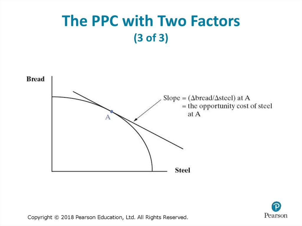
10. The PPC with Two Factors (1 of 3)
• The Ricardian model of Chapter 3 assumed one homogenous inputwith a constant tradeoff between the two goods.
– Complete specialization.
• The HO Model assumes two inputs and different input
requirements for each good.
– Steel takes more capital, less labor.
– Bread takes more labor, less capital.
• This produces a PPC that is convex.
– The opportunity cost increases when we produce more of one good
because we are moving inputs that are less suited to the good with
expanding output.
– Incomplete specialization.
Copyright © 2018 Pearson Education, Ltd. All Rights Reserved.
11. The PPC with Two Factors (2 of 3)
Copyright © 2018 Pearson Education, Ltd. All Rights Reserved.12. The PPC with Two Factors (3 of 3)
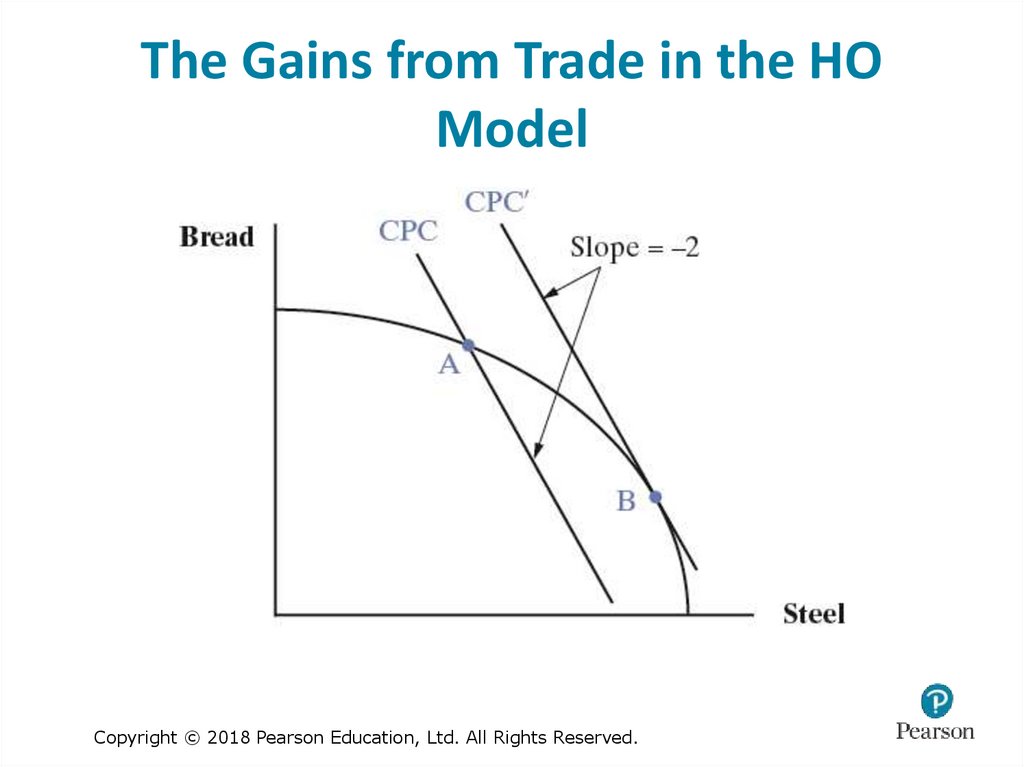
Copyright © 2018 Pearson Education, Ltd. All Rights Reserved.13. The Gains from Trade in the HO Model
Copyright © 2018 Pearson Education, Ltd. All Rights Reserved.14. Income Distribution Effects of Trade in the HO Model (1 of 3)
• Ricardian Model: Every individual benefits fromtrade.
– One input, labor.
– Labor is homogeneous and moves without friction
between sectors.
• HO Model: Not every factor of production
benefits.
– Two inputs, labor and capital
– Owners of labor or capital may be harmed, depending
on which output shrinks when trade begins.
Copyright © 2018 Pearson Education, Ltd. All Rights Reserved.
15. Income Distribution Effects of Trade in the HO Model (2 of 3)
• Trade moves an economy along its PPC, increasingoutput of one good, shrinking output of the other.
• Income for owners of capital and labor depends on
how much demand there is for their services.
– This is called derived demand.
• The demand for their services depends on what is
produced.
– In the bread and steel example, the US increased output of
steel which uses more capital, less labor.
– The incomes of both factors will be affected.
Copyright © 2018 Pearson Education, Ltd. All Rights Reserved.
16. Income Distribution Effects of Trade in the HO Model (3 of 3)
• In our example, the price of steel increased in the US, breadfell. The opposite was true in Canada.
• The Stolper-Samuelson Theorem:
– An increase in the price of a good raises the income of the
factor used intensively in its production.
– A decrease in the price of a good lowers the income of the
factor used intensively in its production.
• US: returns on capital increase, wages fall.
• Canada: returns on capital fall, wages rise.
Copyright © 2018 Pearson Education, Ltd. All Rights Reserved.
17. Income Distribution in the Short Run (1 of 2)
• The HO Model as presented describes the long run,after all changes have worked through the economy.
– We assumed workers and capital owners could effortlessly
move from bread to steel and back, as needed.
– In the short run, however, they may be stuck.
• The Specific Factors Model describes what happens.
– Three factors: Land, Labor, and Capital.
– Two outputs: bread and steel.
– One factor is specific to each output:
Bread is made with labor and land.
Steel is made with labor and capital.
Copyright © 2018 Pearson Education, Ltd. All Rights Reserved.
18. Income Distribution in the Short Run (2 of 2)
• After trade begins:– US landowners see a decline in the demand for land, incomes
fall. Owners of the specific factor used intensively in the
declining industry are hurt.
– US capital owners see an increase in demand for capital,
incomes rise. Owners of the specific factor used intensively in
the expanding industry are better off.
– Labor?
Some move from bread to steel, but since steel is not labor intensive,
their wages fall (same as HO).
However, bread is cheaper, they are better off in that way.
Steel is more expensive, they are worse off from that.
Net result is indeterminate.
Copyright © 2018 Pearson Education, Ltd. All Rights Reserved.
19. Case Study: Comparative Advantage in a Single Natural Resource (1 of 2)
CountryVenezuela
Saudi Arabia
Canada
Iran
Iraq
Kuwait
UAE
Russia
Libya
Nigeria
Reserves
(2015, billions of barrels)
298
268
172
158
144
104
98
80
48
37
(Fuel Exports / Total Exports) x
100 (2013)
96.7
80.6
27.0
60.4
99.6
90.7
30.0
63.6
96.3
79.3
Copyright © 2018 Pearson Education, Ltd. All Rights Reserved.
20. Case Study: Comparative Advantage in a Single Natural Resource (2 of 2)
• The resource curse: The abundant endowment ofa single valuable resource can crowd out other
economic activities.
– Labor and capital become concentrated in the
production of the resource because it is so valuable. It
is hard to develop alternative industries.
– In countries with weak institutions, fighting over the
gains from the resource hinders economic
development.
• The resource curse is not inevitable: see Canada.
Copyright © 2018 Pearson Education, Ltd. All Rights Reserved.
21. Empirical Tests of the Theory of Comparative Advantage
• Tests of the Ricardian Model are relatively successful inpredicting export patterns.
– In this model trade is driven by productivity differences.
• Tests of the factor endowment (HO) model of trade yield
mixed results.
– Empirical tests are difficult: How to measure factor
endowments? Prices in autarky?
– Trade is also affected by technological differences. We assumed
the same technology in the two trading economies but in
reality, different countries have different technologies.
– Other factors are also important: economies of scale, corporate
structures, economic policies.
Copyright © 2018 Pearson Education, Ltd. All Rights Reserved.
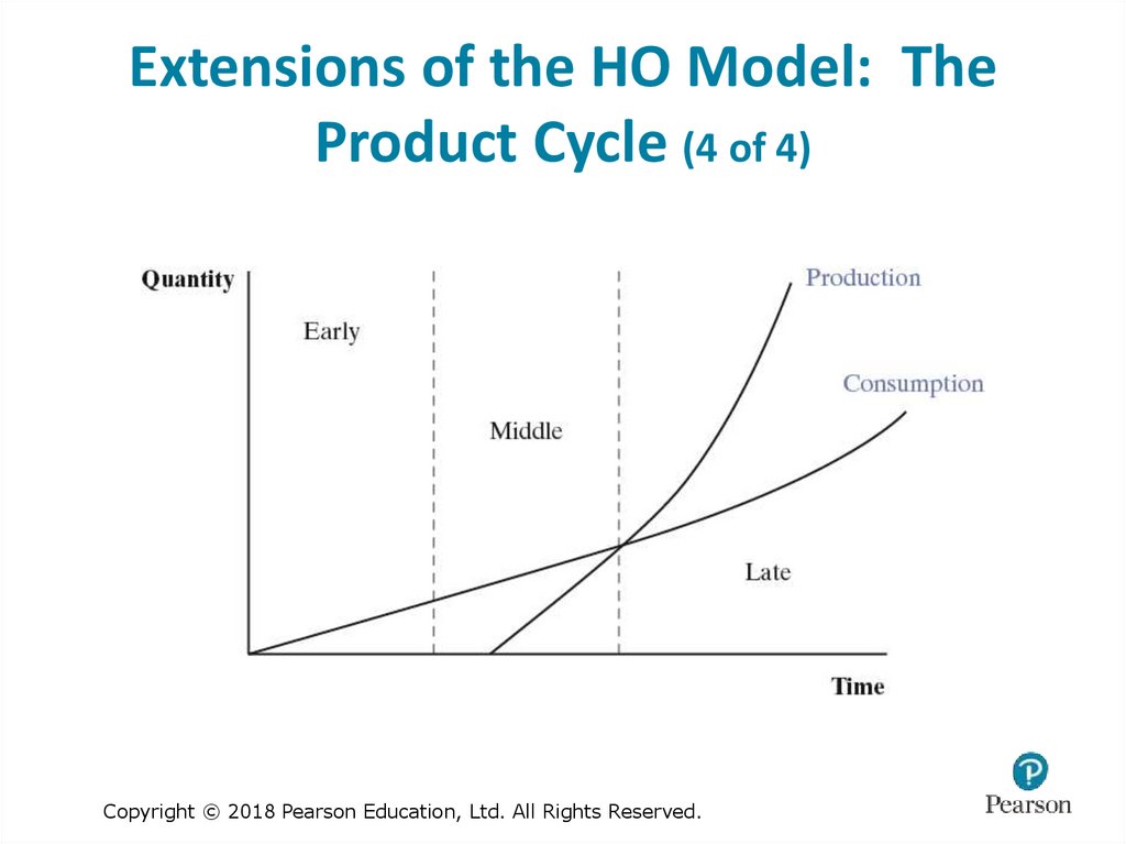
22. Extensions of the HO Model: The Product Cycle (1 of 4)
• The product cycle describes how productionmigrates from high income, advanced economies
to middle income developing economies.
• Early stage of production: Locate in high income
country.
– Need science and engineering skills to develop new
product.
– Need high income consumers to try it out, provide
feedback.
Copyright © 2018 Pearson Education, Ltd. All Rights Reserved.
23. Extensions of the HO Model: The Product Cycle (2 of 4)
• Middle stage of production, location begins toshift.
– Design and production processes beginning to be
standardized.
– Mass production beginning.
– Labor costs begin to matter more.
• Late stage:
– Production moves where labor costs are low.
– The product is completely standardized.
Copyright © 2018 Pearson Education, Ltd. All Rights Reserved.
24. Extensions of the HO Model: The Product Cycle (3 of 4)
Copyright © 2018 Pearson Education, Ltd. All Rights Reserved.25. Extensions of the HO Model: The Product Cycle (4 of 4)
Copyright © 2018 Pearson Education, Ltd. All Rights Reserved.26. Case Study: China’s Top 10 Exports to the U.S. (1 of 2)
ItemCell phones and other household
goods
Computers
Computer accessories
Toys, games, and sporting goods
Apparel, textiles, nonwool or cotton
Telecommunications equipment
Furniture, household goods, etc.
Apparel, household goods—cotton
Footwear
Other parts and accessories of
vehicles
Copyright © 2018 Pearson Education, Ltd. All Rights Reserved.
Millions of $U.S.
64,074
46,091
31,181
25,608
22,957
22,454
16,705
14,413
14,294
13,392
27. Case Study: China’s Top 10 Exports to the U.S. (2 of 2)
• The product cycle and China’s labor endowmentexplain many of their top exports to the U.S.
– Standardized production: cell phones, computers,
telecommunications equipment.
– Labor intensive production: toys, games, sporting
goods, furniture, apparel, footwear.
• Over time, China moves up the ladder of
comparative advantage, producing more capital
intensive and skilled labor intensive goods.
Copyright © 2018 Pearson Education, Ltd. All Rights Reserved.
28. Extension of the HO Model: Investing versus Trading (1 of 4)
• In the HO Model, countries export one thing,import something different.
• In the product cycle, firms invest abroad and
some output may be sent back home.
– A significant share of imports are intrafirm trade:
Trade within one firm.
– In the mid-1990s, around 1/3 of U.S. goods
exports and 2/5ths of imports were intrafirm.
Copyright © 2018 Pearson Education, Ltd. All Rights Reserved.
29. Extension of the HO Model: Investing versus Trading (2 of 4)
• The OLI theory explains why firms choose toinvest abroad instead of trading.
– O: Ownership of an asset that makes a firm
competitive, e.g., technology, trademark, reputation,
etc.
– L: Location abroad offers some advantage, such as
proximity to markets, lower production costs, etc.
– I: Internalization of the advantage instead of
subcontracting or selling the right to produce the
product.
Copyright © 2018 Pearson Education, Ltd. All Rights Reserved.
30. Extension of the HO Model: Investing versus Trading (3 of 4)
• Outsourcing refers to moving some part ofproduction to another firm, either inside the
home country or outside.
• Off-shoring refers to moving some or all of
production abroad.
– If a firm off-shores but does not outsource, it is
working with a foreign affiliate.
– All combinations of off-shoring and outsourcing are
possible.
Copyright © 2018 Pearson Education, Ltd. All Rights Reserved.
31. Extension of the HO Model: Investing versus Trading (4 of 4)
• Modern telecommunications and transportationmake off-shoring easier today.
• This heightens worries about the effects of offshoring.
– The loss of manufacturing jobs.
– Technology theft (non-enforcement of patents, etc.)
– Services might be next: medical services,
accounting, IT, etc., delivered over the internet.
Copyright © 2018 Pearson Education, Ltd. All Rights Reserved.
32. Extension of the HO Model: Internationally Mobile Labor (1 of 2)
• The HO Model assumes that workers cannot move across internationalborders.
• In 2013, there were an estimated 231 million international migrants.
– 20 percent were in the U.S.
– Two-thirds were in high income countries.
• In theory, labor inflows can influence comparative advantage by
changing the labor endowment.
– In the U.S. in the 1980s, the inflow of low skilled immigrants from Central
America caused growth in California’s apparel sector.
– U.S. agriculture relies on immigrant workers.
– Immigrants in some countries work mainly in sectors producing non-traded
goods—construction, nursing, etc.
Copyright © 2018 Pearson Education, Ltd. All Rights Reserved.
33. Extension of the HO Model: Internationally Mobile Labor (1 of 2)
• Economic analysis of migration relies onthree dominant factors:
– Demand pull factors: Pull migrants in (jobs,
higher wages, promises of a better life, etc.)
– Supply push factors: Push migrants out of their
home country (poverty, wars, persecution, etc.)
– Social networks: Determine where they settle in
the receiving country (where there are family,
friends, community members from home).
Copyright © 2018 Pearson Education, Ltd. All Rights Reserved.
34. Trade, Wages, and Jobs (1 of 4)
• The industry and location of jobs (kinds of jobs)may be affected by trade.
– Moving along a PPC.
– There may be short run effects on jobs in particular
industries.
• The overall number of jobs is not determined by
trade; other factors are far more important.
– Fiscal and monetary policies.
– Labor market policies.
Copyright © 2018 Pearson Education, Ltd. All Rights Reserved.
35. Trade, Wages, and Jobs (2 of 4)
• Manufacturing is the most discussed case.– Productivity increases reduce the need for labor.
– Services and manufactured goods production expand
with income, but more and more labor ends up in
services because its productivity does not rise as fast
as in manufacturing.
• Much more manufacturing production today is
exposed to international competition.
– Growth of China and other emerging economies.
– Transportation and telecommunications revolutions.
Copyright © 2018 Pearson Education, Ltd. All Rights Reserved.
36. Trade, Wages, and Jobs (3 of 4)
• Q: Does trade with emerging markets causewages to fall in high income economies?
• A: Economists are not certain.
– Trade may play some role in wage stagnation in
advanced economies.
– But it is also possible that it has little or no effect.
– Many possibilities: For example, automation
reduced the need for labor in manufacturing.
– We need more research on this topic.
Copyright © 2018 Pearson Education, Ltd. All Rights Reserved.
37. Trade, Wages, and Jobs (4 of 4)
• Suppose trade causes jobs to be lost at home,wages to fall. What should we do?
• Options:
– Stop trading and block off-shoring;
– Selectively block imports and off-shoring;
– Keep trading and investing but assist workers.
– Do nothing.
• Each option has costs and benefits.
Copyright © 2018 Pearson Education, Ltd. All Rights Reserved.














 economics


