


 economics
Similar presentations:


")


Lecture # 09. Inputs and Production Functions
1.
Lecture # 09Inputs and Production Functions
Lecturer: Martin Paredes
2.
1. The Production FunctionMarginal and Average Products
Isoquants
Marginal Rate of Technical Substitution
2. Returns to Scale
3. Some Special Functional Forms
4. Technological Progress
2
3.
1. Inputs or factors of production areproductive resources that firms use to
manufacture goods and services.
Example: labor, land, capital
equipment…
2. The firm’s output is the amount of goods
and services produced by the firm.
3
4.
3. Production transforms a set of inputsinto a set of outputs
4. Technology determines the quantity of
output that is feasible to attain for a given
set of inputs.
4
5.
5. The production function tells us themaximum possible output that can be
attained by the firm for any given
quantity of inputs.
Q = F(L,K,T,M,…)
5
6.
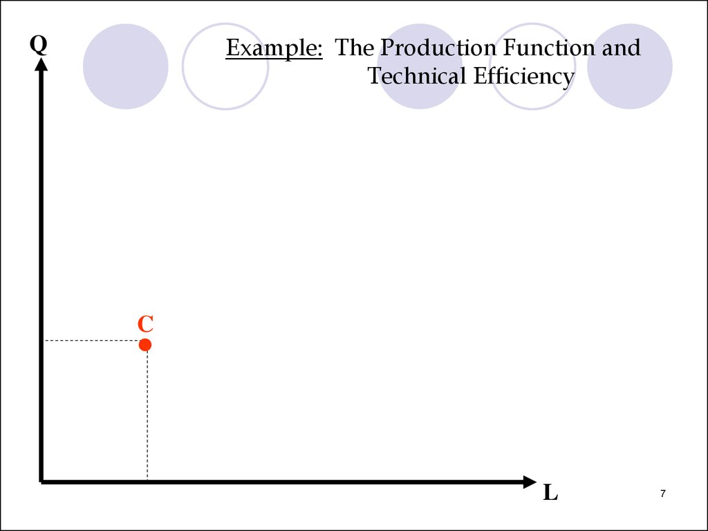
6. A technically efficient firm is attaining themaximum possible output from its inputs
(using whatever technology is appropriate)
7. The firm’s production set is the set of all
feasible points, including:
The production function (efficient point)
The inefficient points below the production
function
6
7.
Example: The Production Function andTechnical Efficiency
Q
C
L
7
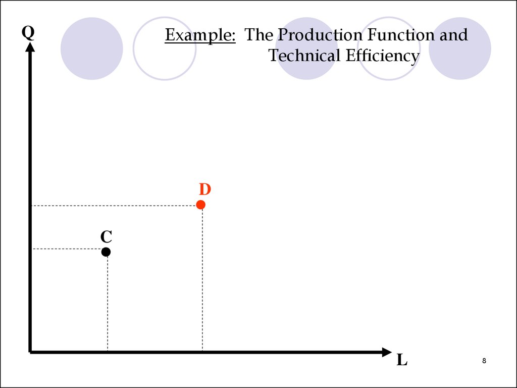
8.
Example: The Production Function andTechnical Efficiency
Q
D
C
L
8
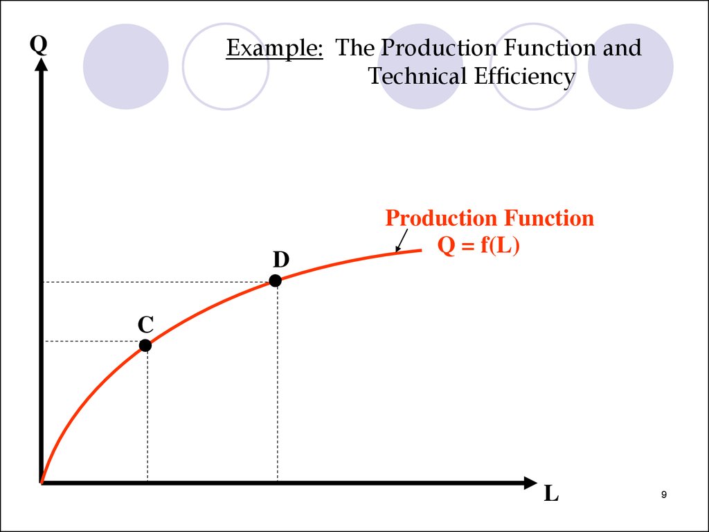
9.
Example: The Production Function andTechnical Efficiency
Q
D
Production Function
Q = f(L)
C
L
9
10.
Example: The Production Function andTechnical Efficiency
Q
D
C
•A
•B
Production Function
Q = f(L)
L
10
11.
Example: The Production Function andTechnical Efficiency
Q
D
C
•A
•B
Production Function
Q = f(L)
Production Set
L
11
12.
Notes:The variables in the production function are
flows (amount of input per unit of time), not
stocks (the absolute quantity of the input).
Capital refers to physical capital (goods that
are themselves produced goods) and not
financial capital (money required to start or
maintain production).
12
13.
Utility FunctionSatisfaction from
purchases
Production Function
Output from inputs
2.
Derived from
preferences
Derived from
technologies
3.
Ordinal
Cardinal
1.
13
14.
4.Utility Function
Marginal Utility
5. Indifference Curves
6.
Marginal Rate of
Substitution
Production Function
Marginal Product
Isoquants
Marginal Rate of
Technical Substitution
14
15.
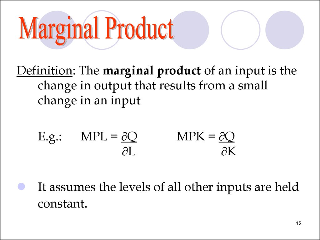
Definition: The marginal product of an input is thechange in output that results from a small
change in an input
E.g.:
MPL = Q
L
MPK = Q
K
It assumes the levels of all other inputs are held
constant.
15
16.
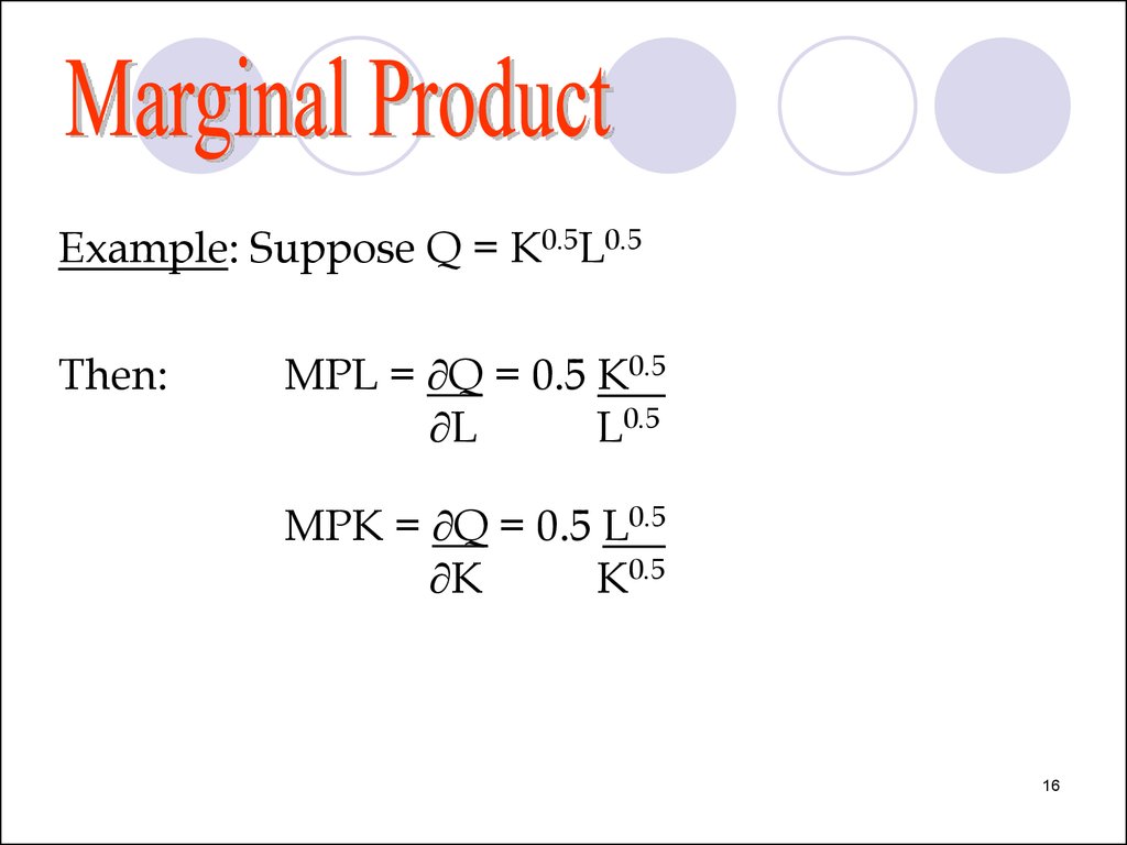
Example: Suppose Q = K0.5L0.5Then:
MPL = Q = 0.5 K0.5
L
L0.5
MPK = Q = 0.5 L0.5
K
K0.5
16
17.
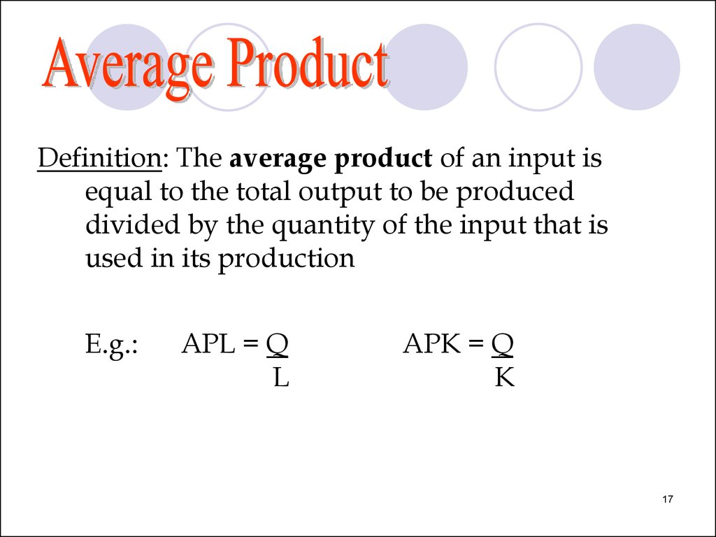
Definition: The average product of an input isequal to the total output to be produced
divided by the quantity of the input that is
used in its production
E.g.:
APL = Q
L
APK = Q
K
17
18.
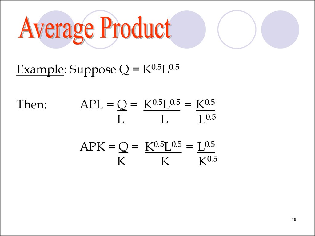
Example: Suppose Q = K0.5L0.5Then:
APL = Q = K0.5L0.5 = K0.5
L
L
L0.5
APK = Q = K0.5L0.5 = L0.5
K
K
K0.5
18
19.
Definition: The law of diminishing marginalreturns states that the marginal product
(eventually) declines as the quantity used of a
single input increases.
19
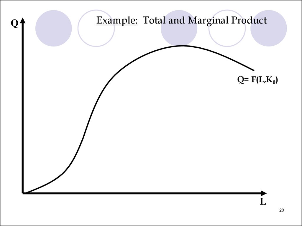
20.
QExample: Total and Marginal Product
Q= F(L,K0)
L
20
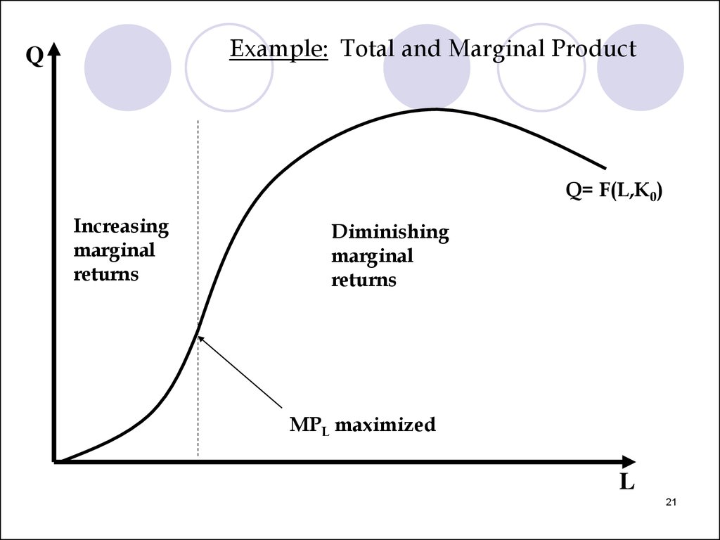
21.
Example: Total and Marginal ProductQ
Q= F(L,K0)
Increasing
marginal
returns
Diminishing
marginal
returns
MPL maximized
L
21
22.
QExample: Total and Marginal Product
Q= F(L,K0)
MPL = 0 when
TP maximized
Increasing
total returns
Diminishing
total returns
L
22
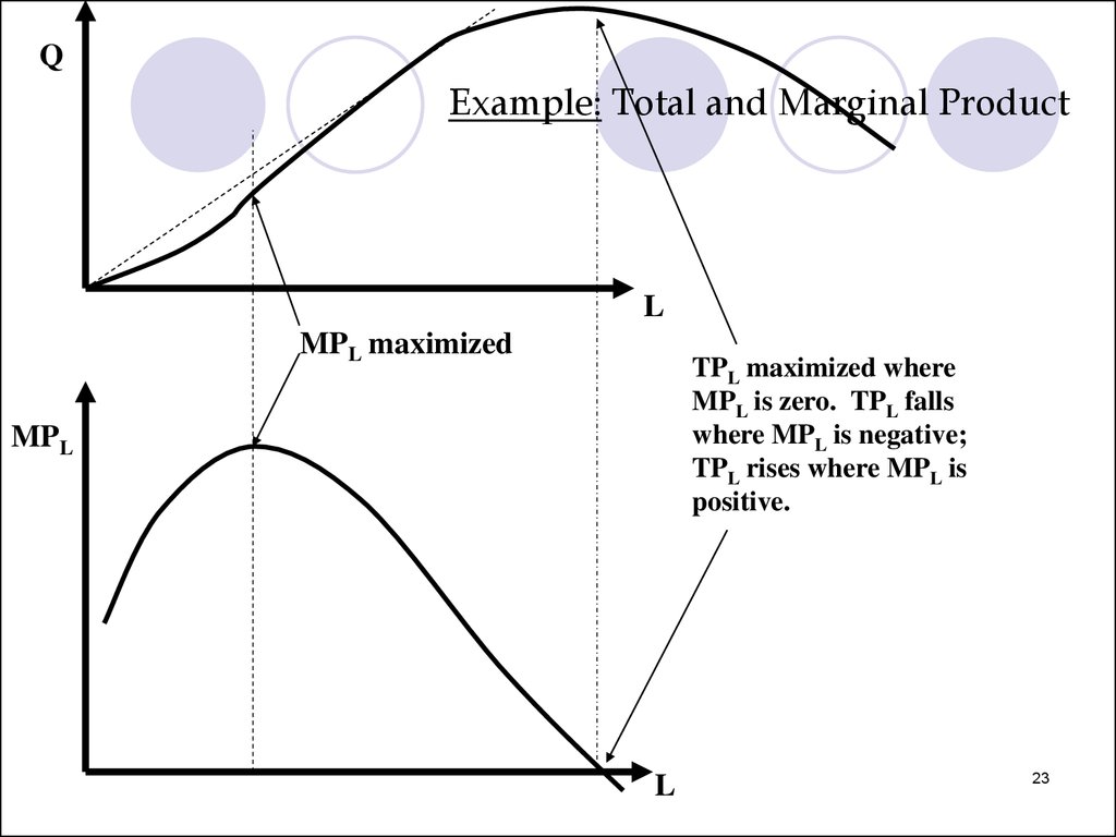
23.
QExample: Total and Marginal Product
L
MPL maximized
TPL maximized where
MPL is zero. TPL falls
where MPL is negative;
TPL rises where MPL is
positive.
MPL
L
23
24.
There is a systematic relationship betweenaverage product and marginal product.
This relationship holds for any comparison
between any marginal magnitude with the
average magnitude.
24
25.
1. When marginal product is greater than averageproduct, average product is increasing.
E.g., if MPL > APL , APL increases in L.
2. When marginal product is less than average
product, average product is decreasing.
E.g., if MPL < APL, APL decreases in L.
25
26.
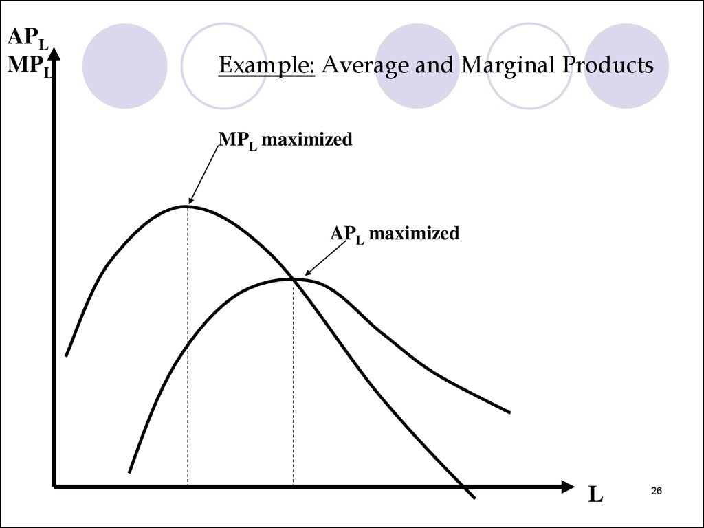
APLMPL
Example: Average and Marginal Products
MPL maximized
APL maximized
L
26
27.
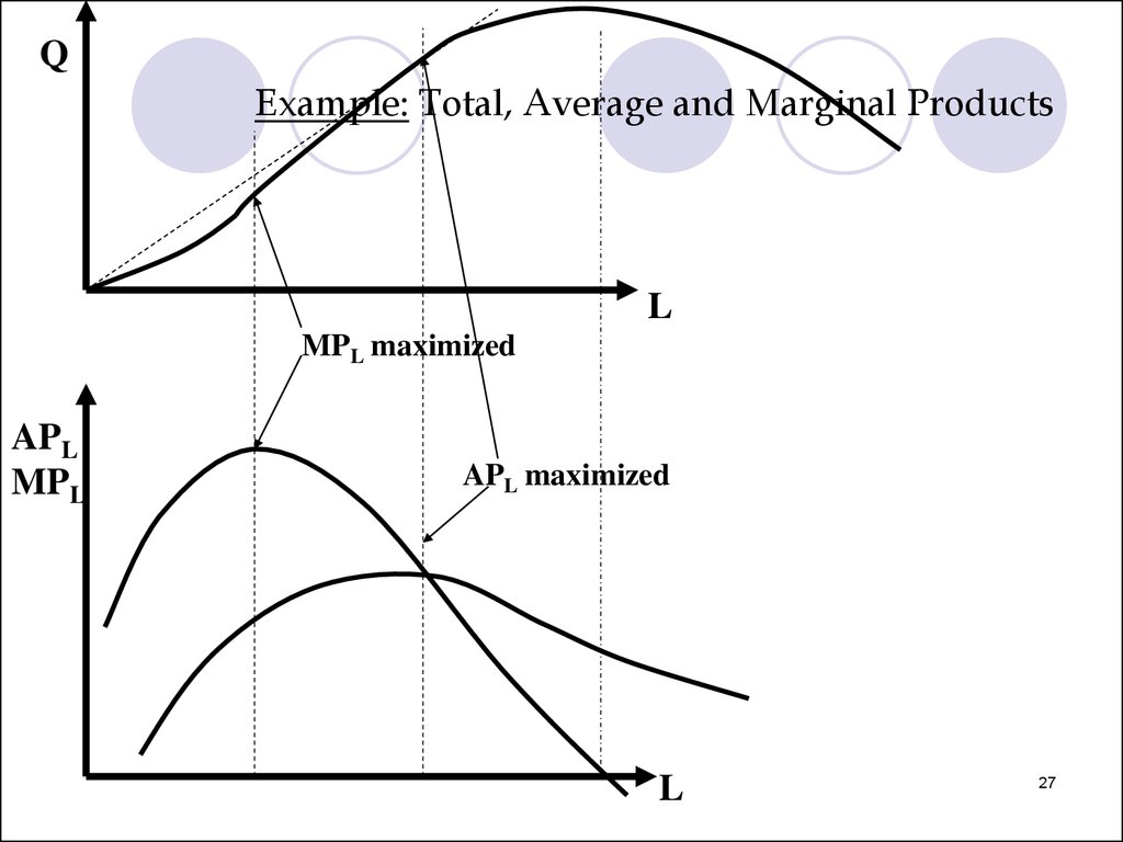
QExample: Total, Average and Marginal Products
L
MPL maximized
APL
MPL
APL maximized
L
27
28.
Definition: An isoquant is a representation of allthe combinations of inputs (labor and capital)
that allow that firm to produce a given quantity
of output.
28
29.
KExample: Isoquants
Slope=dK/dL
0
Q = 10
L
L
29
30.
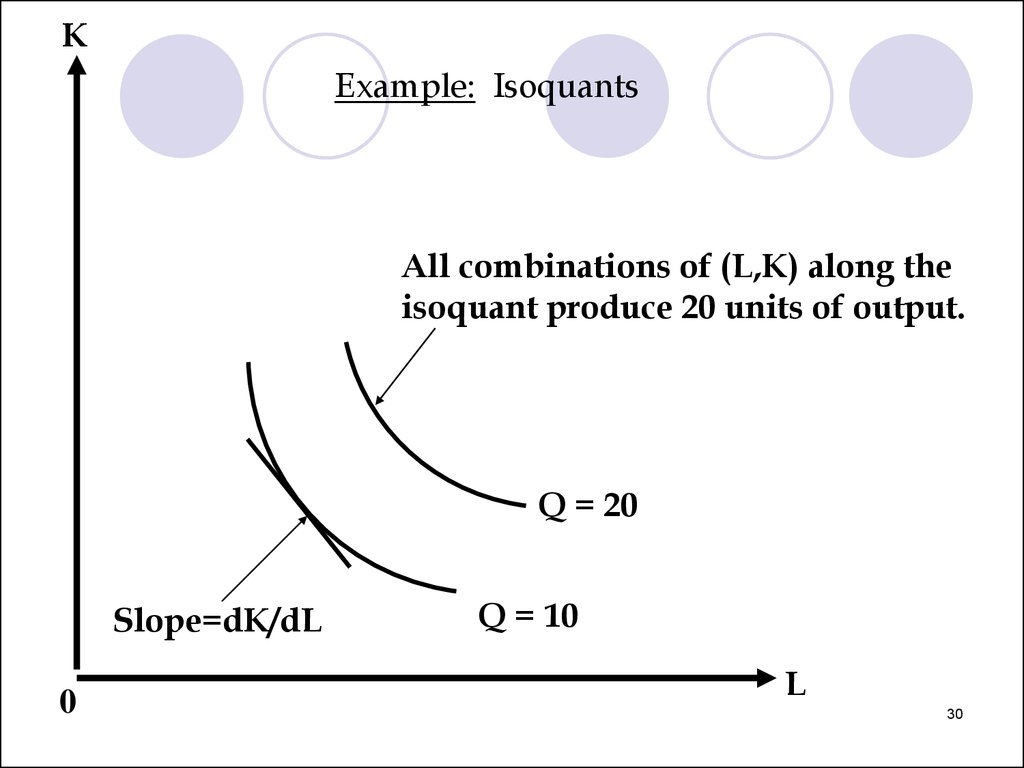
KExample: Isoquants
All combinations of (L,K) along the
isoquant produce 20 units of output.
Q = 20
Slope=dK/dL
0
Q = 10
L
30
31.
Example: Suppose Q = K0.5L0.5For Q = 20
=> 20 = K0.5L0.5
=> 400 = KL
=> K = 400/L
For Q = Q0
=> K = (Q0)2 /L
31
32.
Definition: The marginal rate of technicalsubstitution measures the rate at which the
firm can substitute a little more of an input for a
little less of another input, in order to produce the
same output as before.
32
33.
Alternative Definition : It is the negative of the slopeof the isoquant:
MRTSL,K = — dK (for a constant level of
dL
output)
33
34.
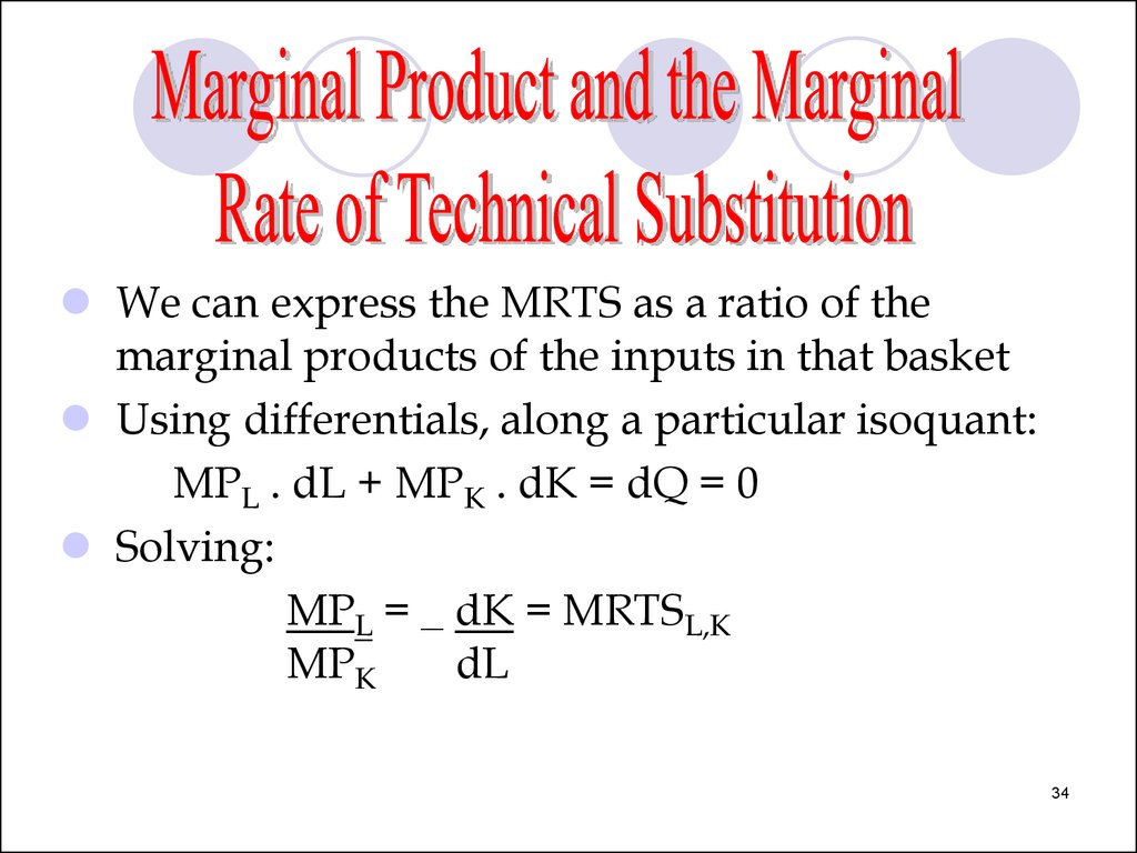
We can express the MRTS as a ratio of themarginal products of the inputs in that basket
Using differentials, along a particular isoquant:
MPL . dL + MPK . dK = dQ = 0
Solving:
MPL = _ dK = MRTSL,K
MPK
dL
34
35.
Notes:If we have diminishing marginal returns, we also
have a diminishing marginal rate of technical
substitution.
In other words, the marginal rate of technical
substitution of labour for capital diminishes as
the quantity of labour increases along an
isoquant.
35
36.
Notes:If both marginal products are positive, the slope
of the isoquant is negative
For many production functions, marginal
products eventually become negative. Then:
MRTS < 0
We reach an uneconomic region of production
36
37.
KExample: The Economic and the
Uneconomic Regions of Production
Isoquants
Q = 20
Q = 10
0
L
37
38.
KExample: The Economic and the
Uneconomic Regions of Production
A
B
Q = 20
Q = 10
0
L
38
39.
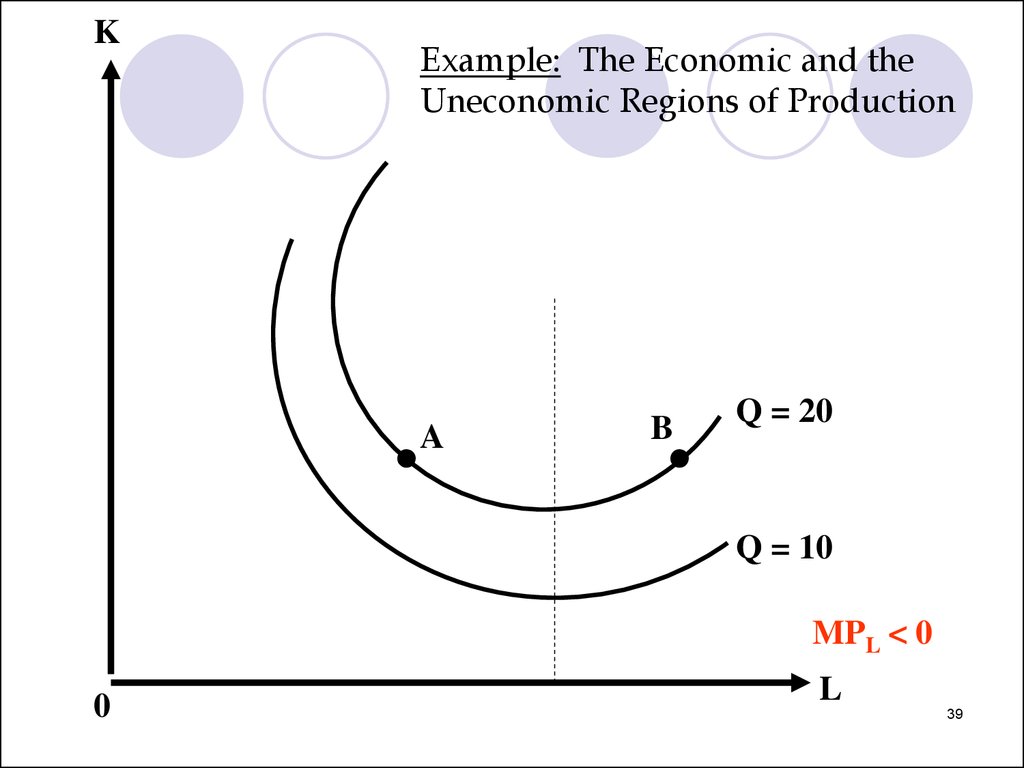
KExample: The Economic and the
Uneconomic Regions of Production
A
B
Q = 20
Q = 10
MPL < 0
0
L
39
40.
KExample: The Economic and the
Uneconomic Regions of Production
MPK < 0
A
B
Q = 20
Q = 10
MPL < 0
0
L
40
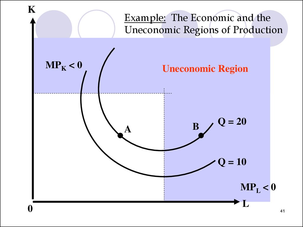
41.
KExample: The Economic and the
Uneconomic Regions of Production
MPK < 0
Uneconomic Region
A
B
Q = 20
Q = 10
MPL < 0
0
L
41
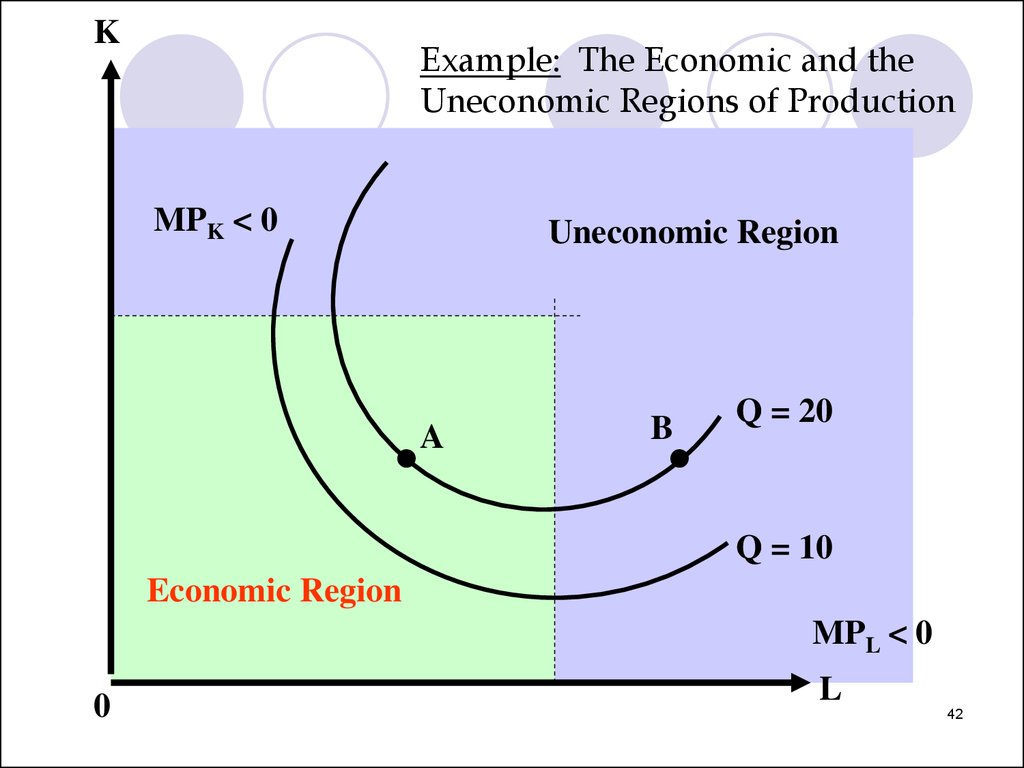
42.
KExample: The Economic and the
Uneconomic Regions of Production
MPK < 0
Uneconomic Region
A
B
Q = 20
Q = 10
Economic Region
MPL < 0
0
L
42