Specific factors model

1. Lecture 3

Lecture 3
Specific Factors
and Income
Distribution
•© Pearson Education Limited 2015. All rights reserved.
•1-1

2. Chapter Organization

• Introduction
• The Specific Factors Model
• International Trade in the Specific Factors
Model
• Income Distribution and the Gains from
Trade
• Political Economy of Trade: A Preliminary
View
• International Labor Mobility
• Summary
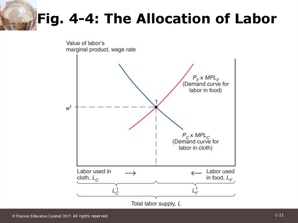
•© Pearson Education Limited 2015. All rights reserved.
•1-2

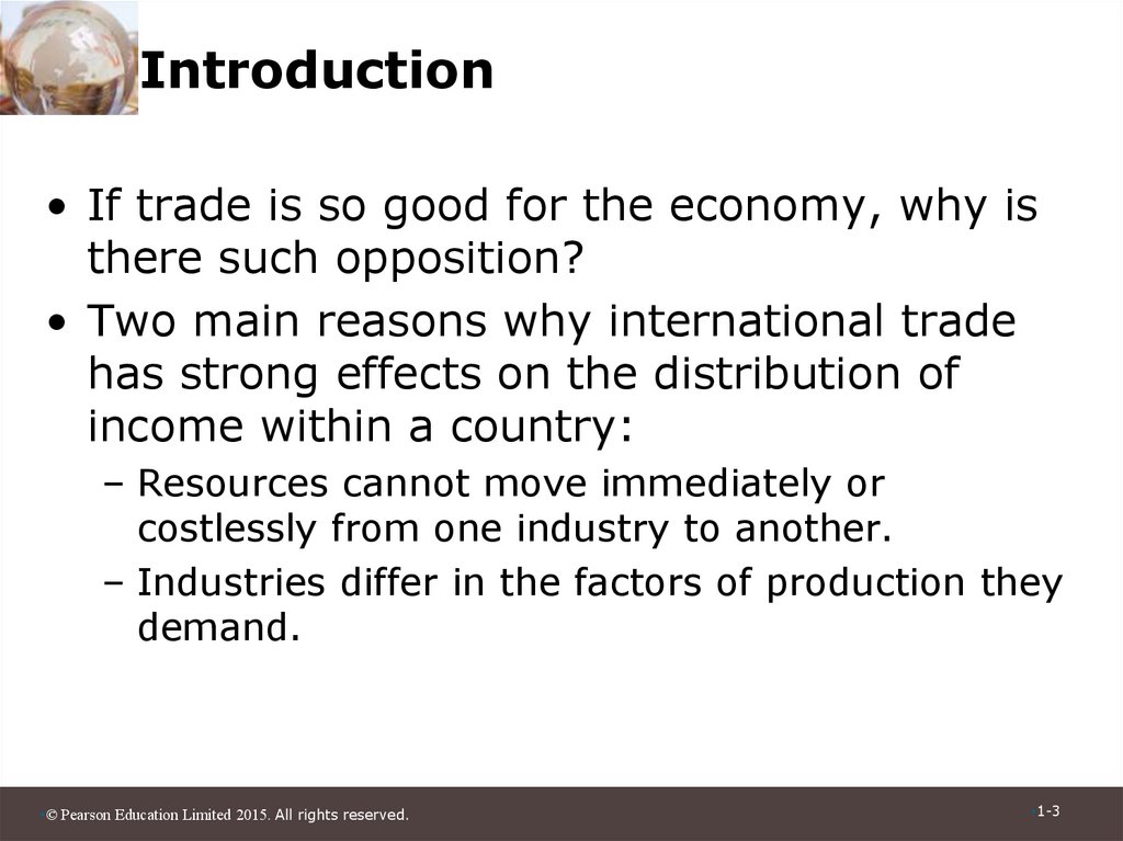
3. Introduction

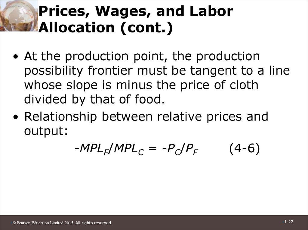
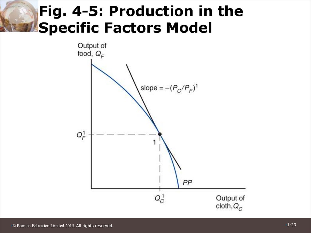
• If trade is so good for the economy, why is
there such opposition?
• Two main reasons why international trade
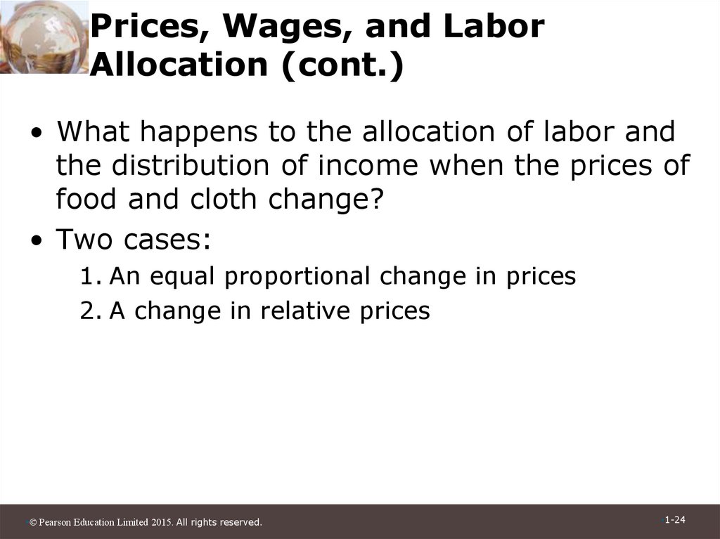
has strong effects on the distribution of
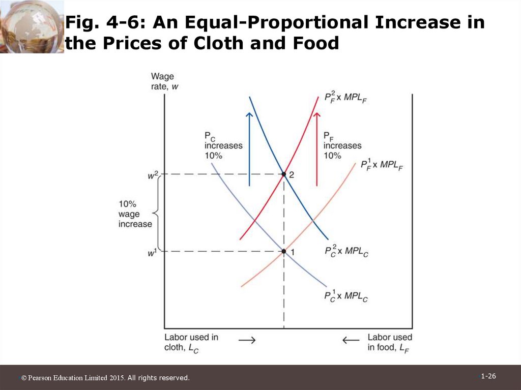
income within a country:
– Resources cannot move immediately or
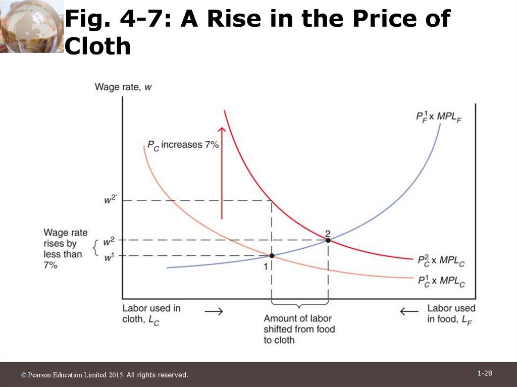
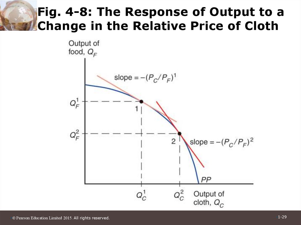
costlessly from one industry to another.
– Industries differ in the factors of production they
demand.
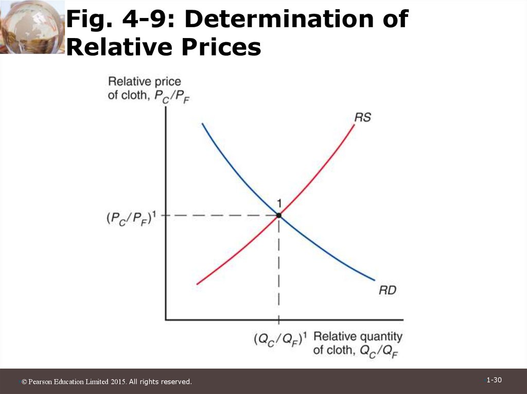
•© Pearson Education Limited 2015. All rights reserved.
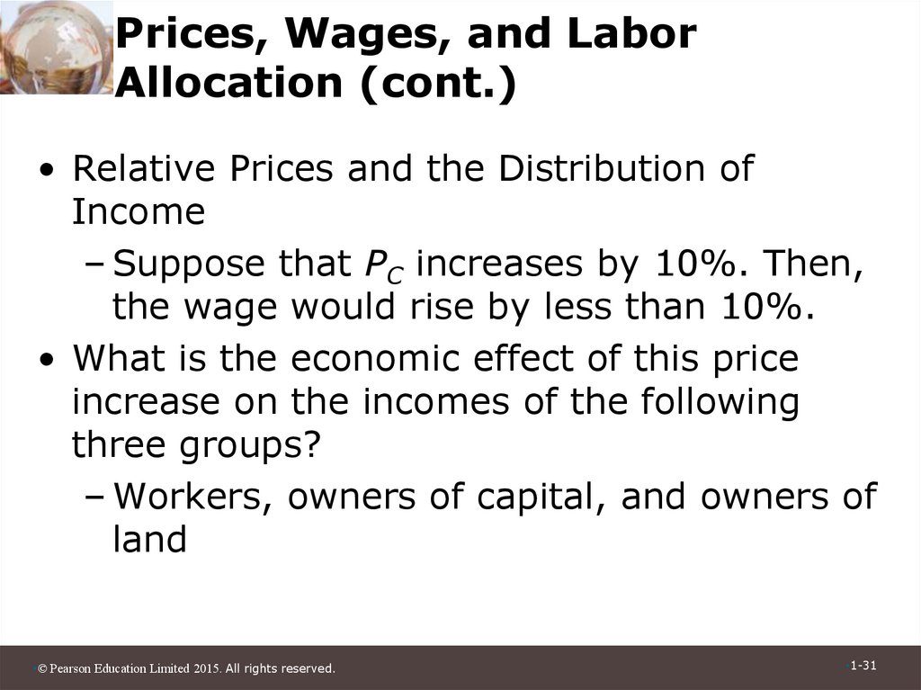
•1-3

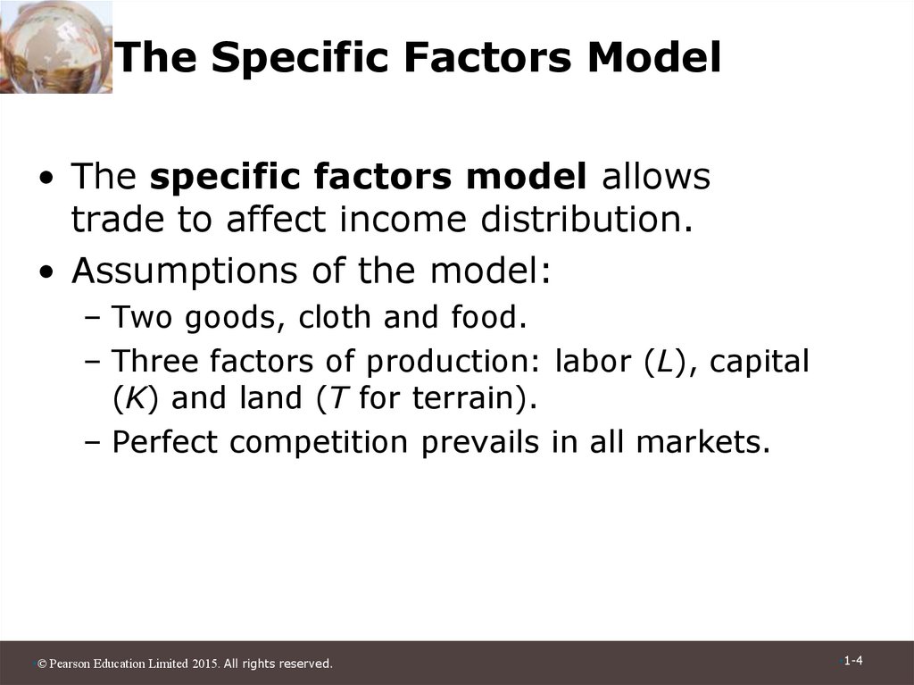
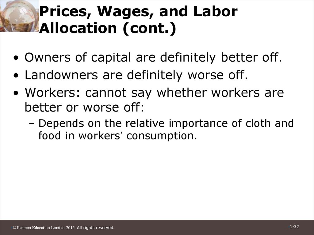
4. The Specific Factors Model

• The specific factors model allows
trade to affect income distribution.
• Assumptions of the model:
– Two goods, cloth and food.
– Three factors of production: labor (L), capital
(K) and land (T for terrain).
– Perfect competition prevails in all markets.
•© Pearson Education Limited 2015. All rights reserved.
•1-4

5. The Specific Factors Model (cont.)

– Cloth produced using capital and labor (but not
land).
– Food produced using land and labor (but not
capital).
– Labor is a mobile factor that can move between
sectors.
– Land and capital are both specific factors used
only in the production of one good.
•© Pearson Education Limited 2015. All rights reserved.
•1-5

6. The Specific Factors Model (cont.)

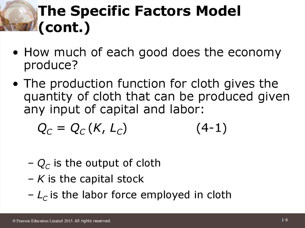
• How much of each good does the economy
produce?
• The production function for cloth gives the
quantity of cloth that can be produced given
any input of capital and labor:
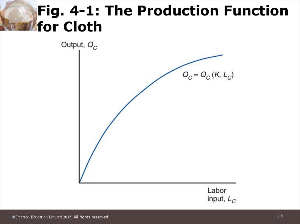
QC = QC (K, LC)
(4-1)
– QC is the output of cloth
– K is the capital stock
– LC is the labor force employed in cloth
•© Pearson Education Limited 2015. All rights reserved.
•1-6

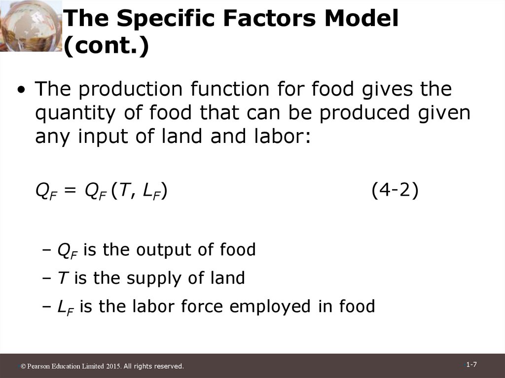
7. The Specific Factors Model (cont.)

• The production function for food gives the
quantity of food that can be produced given
any input of land and labor:
QF = QF (T, LF)
(4-2)
– QF is the output of food
– T is the supply of land
– LF is the labor force employed in food
•© Pearson Education Limited 2015. All rights reserved.
•1-7

8. Production Possibilities

• How does the economy’s mix of output
change as labor is shifted from one sector to
the other?
• When labor moves from food to cloth, food
production falls while output of cloth rises.
• Figure 4-1 illustrates the production function
for cloth.
•© Pearson Education Limited 2015. All rights reserved.
•1-8

9. Fig. 4-1: The Production Function for Cloth

•© Pearson Education Limited 2015. All rights reserved.
•1-9

10. Production Possibilities (cont.)

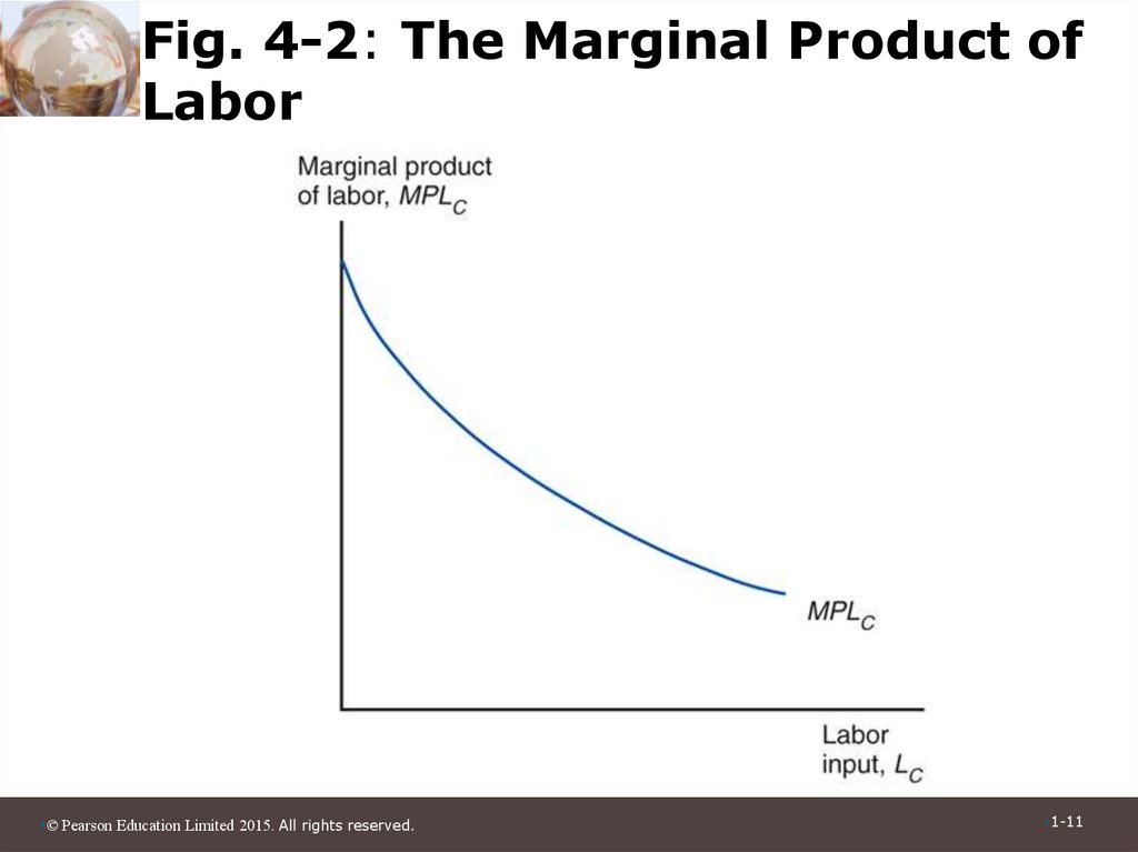
• The shape of the production function reflects
the law of diminishing marginal returns.
– Adding one worker to the production process
(without increasing the amount of capital) means
that each worker has less capital to work with.
– Therefore, each additional unit of labor adds less
output than the last.
• Figure 4-2 shows the marginal product of
labor, which is the increase in output that
corresponds to an extra unit of labor.
•© Pearson Education Limited 2015. All rights reserved.
•1-10

11. Fig. 4-2: The Marginal Product of Labor

•© Pearson Education Limited 2015. All rights reserved.
•1-11

12. Production Possibilities (cont.)

• For the economy as a whole, the total labor
employed in cloth and food must equal the total
labor supply:
LC + LF = L
(4-3)
• Use these equations to derive the production
possibilities frontier of the economy.
•© Pearson Education Limited 2015. All rights reserved.
•1-12

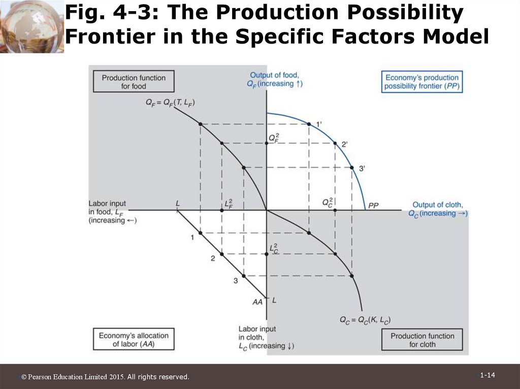
13. Production Possibilities (cont.)

• Use a four-quadrant diagram to construct
production possibilities frontier in Figure 4-3.
– Lower left quadrant indicates the allocation of labor.
– Lower right quadrant shows the production function for
cloth from Figure 4-1.
– Upper left quadrant shows the corresponding production
function for food.
– Upper right quadrant indicates the combinations of cloth
and food that can be produced.
•© Pearson Education Limited 2015. All rights reserved.
•1-13

14. Fig. 4-3: The Production Possibility Frontier in the Specific Factors Model

•© Pearson Education Limited 2015. All rights reserved.
•1-14

15. Production Possibilities (cont.)

• Why is the production possibilities frontier
curved?
– Diminishing returns to labor in each sector cause
the opportunity cost to rise when an economy
produces more of a good.
– Opportunity cost of cloth in terms of food is the
slope of the production possibilities frontier – the
slope becomes steeper as an economy produces
more cloth.
•© Pearson Education Limited 2015. All rights reserved.
•1-15

16. Production Possibilities (cont.)

• Opportunity cost of producing one more
yard of cloth is MPLF/MPLC pounds of food.
– To produce one more yard of cloth, you need
1/MPLC hours of labor.
– To free up one hour of labor, you must reduce
output of food by MPLF pounds.
– To produce less food and more cloth, employ less
in food and more in cloth.
• The marginal product of labor in food rises and the
marginal product of labor in cloth falls, so MPLF/MPLC
rises.
•© Pearson Education Limited 2015. All rights reserved.
•1-16

17. Prices, Wages, and Labor Allocation

• How much labor is employed in each
sector?
– Need to look at supply and demand in the
labor market.
• Demand for labor:
– In each sector, employers will maximize
profits by demanding labor up to the point
where the value produced by an additional
hour equals the marginal cost of employing a
worker for that hour.
•© Pearson Education Limited 2015. All rights reserved.
•1-17

18. Prices, Wages, and Labor Allocation (cont.)

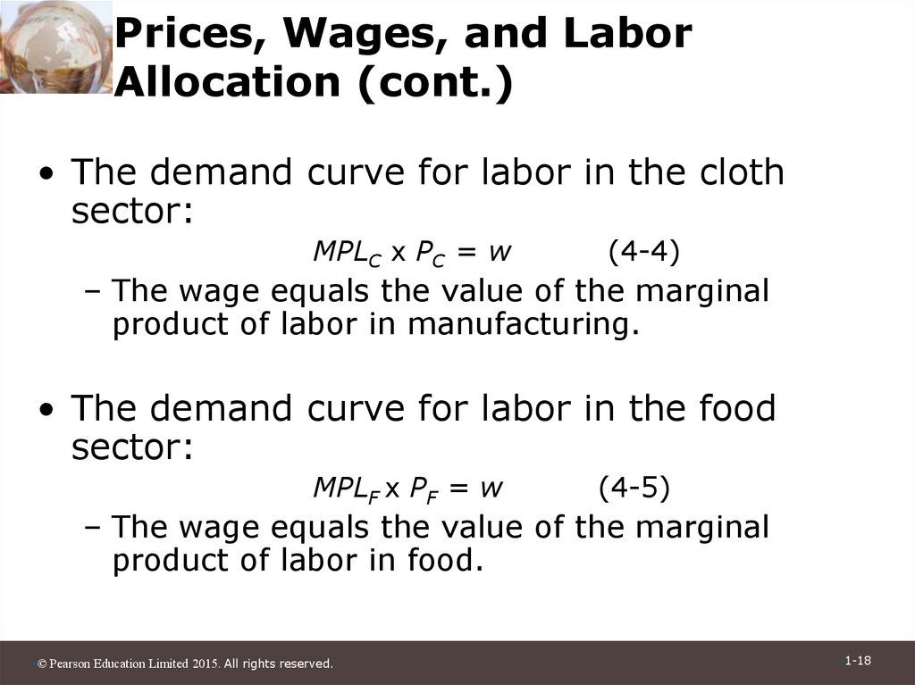
• The demand curve for labor in the cloth
sector:
MPLC x PC = w
(4-4)
– The wage equals the value of the marginal
product of labor in manufacturing.
• The demand curve for labor in the food
sector:
MPLF x PF = w
(4-5)
– The wage equals the value of the marginal
product of labor in food.
•© Pearson Education Limited 2015. All rights reserved.
•1-18

19. Prices, Wages, and Labor Allocation (cont.)

• Figure 4-4 represents labor demand in the
two sectors.
• The demand for labor in the cloth sector is
MPLC from Figure 4-2 multiplied by PC.
• The demand for labor in the food sector is
measured from the right.
• The horizontal axis represents the total
labor supply L.
•© Pearson Education Limited 2015. All rights reserved.
•1-19

20. Prices, Wages, and Labor Allocation (cont.)

• The two sectors must pay the same wage because
labor can move between sectors.
• If the wage were higher in the cloth sector, workers
would move from making food to making cloth until
the wages become equal.
– Or if the wage were higher in the food sector, workers
would move in the other direction.
• Where the labor demand curves intersect gives the
equilibrium wage and allocation of labor between
the two sectors.
•© Pearson Education Limited 2015. All rights reserved.
•1-20

21. Fig. 4-4: The Allocation of Labor

•© Pearson Education Limited 2015. All rights reserved.
•1-21

22. Prices, Wages, and Labor Allocation (cont.)

• At the production point, the production
possibility frontier must be tangent to a line
whose slope is minus the price of cloth
divided by that of food.
• Relationship between relative prices and
output:
-MPLF/MPLC = -PC/PF
(4-6)
•© Pearson Education Limited 2015. All rights reserved.
•1-22

23. Fig. 4-5: Production in the Specific Factors Model

•© Pearson Education Limited 2015. All rights reserved.
•1-23

24. Prices, Wages, and Labor Allocation (cont.)

• What happens to the allocation of labor and
the distribution of income when the prices of
food and cloth change?
• Two cases:
1. An equal proportional change in prices
2. A change in relative prices
•© Pearson Education Limited 2015. All rights reserved.
•1-24

25. Prices, Wages, and Labor Allocation (cont.)

• When both prices change in the same
proportion, no real changes occur.
– The wage rate (w) rises in the same proportion
as the prices, so real wages (i.e., the ratios of
the wage rate to the prices of goods) are
unaffected.
– The real incomes of capital owners and
landowners also remain the same.
•© Pearson Education Limited 2015. All rights reserved.
•1-25

26. Fig. 4-6: An Equal-Proportional Increase in the Prices of Cloth and Food

•© Pearson Education Limited 2015. All rights reserved.
•1-26

27. Prices, Wages, and Labor Allocation (cont.)

• When only PC rises, labor shifts from the
food sector to the cloth sector and the
output of cloth rises while that of food falls.
• The wage rate (w) does not rise as much as
PC since cloth employment increases and
thus the marginal product of labor in that
sector falls.
•© Pearson Education Limited 2015. All rights reserved.
•1-27

28. Fig. 4-7: A Rise in the Price of Cloth

•© Pearson Education Limited 2015. All rights reserved.
•1-28

29. Fig. 4-8: The Response of Output to a Change in the Relative Price of Cloth

•© Pearson Education Limited 2015. All rights reserved.
•1-29

30. Fig. 4-9: Determination of Relative Prices

•© Pearson Education Limited 2015. All rights reserved.
•1-30

31. Prices, Wages, and Labor Allocation (cont.)

• Relative Prices and the Distribution of
Income
– Suppose that PC increases by 10%. Then,
the wage would rise by less than 10%.
• What is the economic effect of this price
increase on the incomes of the following
three groups?
– Workers, owners of capital, and owners of
land
•© Pearson Education Limited 2015. All rights reserved.
•1-31

32. Prices, Wages, and Labor Allocation (cont.)

• Owners of capital are definitely better off.
• Landowners are definitely worse off.
• Workers: cannot say whether workers are
better or worse off:
– Depends on the relative importance of cloth and
food in workers’ consumption.
•© Pearson Education Limited 2015. All rights reserved.
•1-32

33.

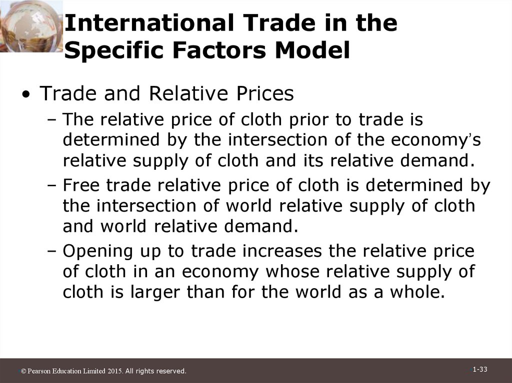
International Trade in the
Specific Factors Model
• Trade and Relative Prices
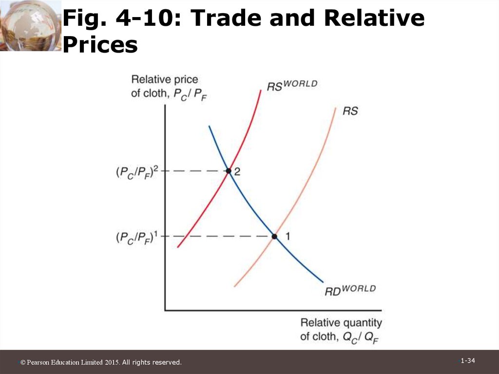
– The relative price of cloth prior to trade is
determined by the intersection of the economy’s
relative supply of cloth and its relative demand.
– Free trade relative price of cloth is determined by
the intersection of world relative supply of cloth
and world relative demand.
– Opening up to trade increases the relative price
of cloth in an economy whose relative supply of
cloth is larger than for the world as a whole.
•© Pearson Education Limited 2015. All rights reserved.
•1-33

34. Fig. 4-10: Trade and Relative Prices

•© Pearson Education Limited 2015. All rights reserved.
•1-34

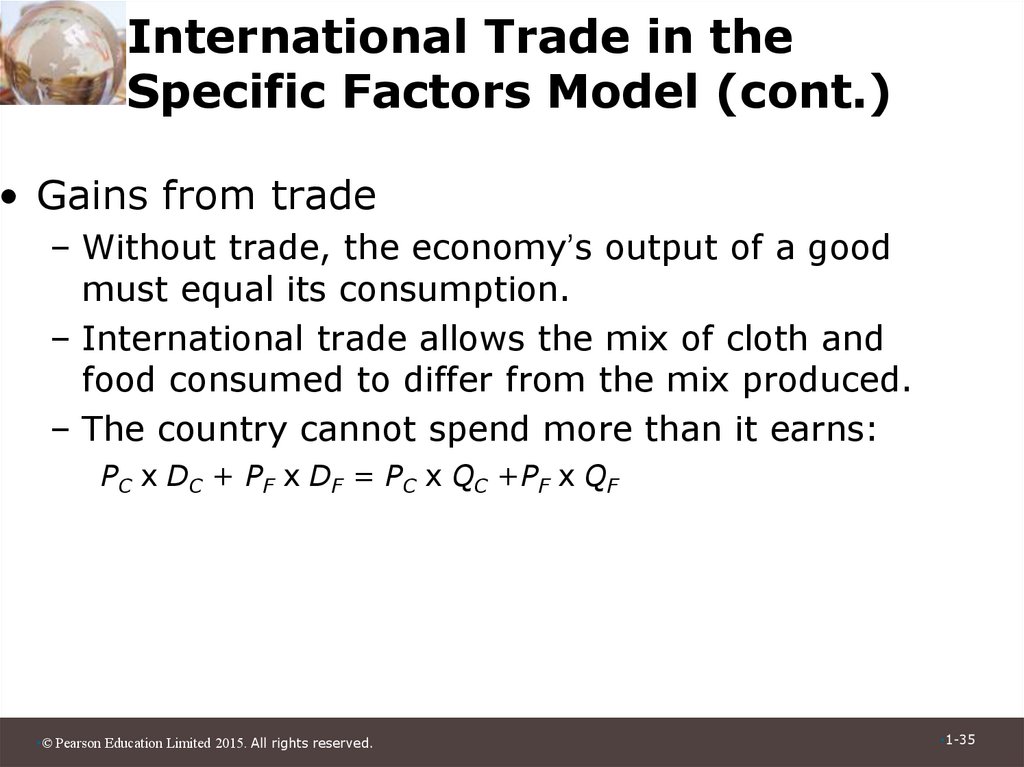
35. International Trade in the Specific Factors Model (cont.)

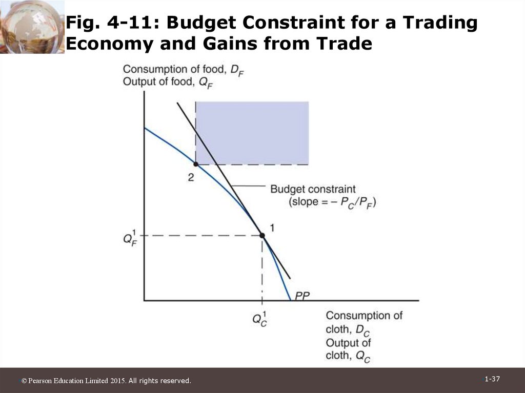
• Gains from trade
– Without trade, the economy’s output of a good
must equal its consumption.
– International trade allows the mix of cloth and
food consumed to differ from the mix produced.
– The country cannot spend more than it earns:
PC x DC + PF x DF = PC x QC +PF x QF
•© Pearson Education Limited 2015. All rights reserved.
•1-35

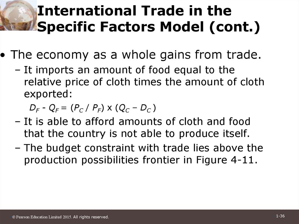
36. International Trade in the Specific Factors Model (cont.)

• The economy as a whole gains from trade.
– It imports an amount of food equal to the
relative price of cloth times the amount of cloth
exported:
DF - QF = (PC / PF) x (QC – DC )
– It is able to afford amounts of cloth and food
that the country is not able to produce itself.
– The budget constraint with trade lies above the
production possibilities frontier in Figure 4-11.
•© Pearson Education Limited 2015. All rights reserved.
•1-36

37. Fig. 4-11: Budget Constraint for a Trading Economy and Gains from Trade

•© Pearson Education Limited 2015. All rights reserved.
•1-37