A New Stainless Steel Tube in Tube Damper for Seismic Protection of Structures 14 стр

1.

A New Stainless Steel Tube in Tube Damper for Seismic Protection of Structures
by https://www.mdpi.com/2076-3417/10/4/1410/htm
Guillermo González-Sanz
,
David Escolano-Margarit
and
Amadeo Benavent-Climent
*
Department of Mechanical Engineering, Universidad Politécnica de Madrid, 28006 Madrid, Spain
*
Author to whom correspondence should be addressed.
Appl. Sci. 2020, 10(4), 1410; https://doi.org/10.3390/app10041410
Received: 1 February 2020 / Revised: 13 February 2020 / Accepted: 17 February 2020 / Published: 19 February
2020
(This article belongs to the Special Issue Passive Seismic Control of Structures with Energy Dissipation
Systems)
Download PDF
Browse Figures
Citation Export
Abstract
This paper investigates a new stainless-steel tube-in-tube damper (SS-TTD) designed for the passive control of
structures subjected to seismic loadings. It consists of two tubes assembled in a telescopic configuration. A series of
slits are cut on the walls of the exterior tube in order to create a series of strips with a large height-to-width ratio. The
exterior tube is connected to the interior tube so that when the brace-type damper is subjected to forced axial
displacements, the strips dissipate energy in the form of flexural plastic deformations. The performance of the SS-TTD
is assessed experimentally through quasi-static and dynamic shaking table tests. Its ultimate energy dissipation
capacity is quantitatively evaluated, and a procedure is proposed to predict the failure. The cumulative ductility of the
SS-TTD is about 4-fold larger than that reported for other dampers based on slit-type plates in previous studies. Its
ultimate energy dissipation capacity is 3- and 16-fold higher than that of slit-type plates made of mild steel and highstrength steel, respectively. Finally, two hysteretic models are investigated and compared to characterise the
hysteretic behaviour of the SS-TTD under arbitrarily applied cyclic loads.
Keywords: metallic damper; stainless steel; shaking table test; cyclic loading; energy dissipation
1. Introduction
For decades, seismic-resistant structures have been designed using the conventional approach of ensuring life
safety against earthquakes, the main objective being to prevent buildings from collapsing. However, this approach
comes at the cost of assuming important damage to the structure after the earthquake, requiring in most cases its
demolition and rebuilding or a high cost of repair. Strong ground motions such as the Northridge (Northridge, 1994) or
1

2.

Hyogo-ken Nambu (Kobe, 1995) earthquakes have long since proven that this approach is no longer valid, as
economic losses are also to be considered in seismic-resistant design. Controlling damage is a key aspect of the socalled Performance-Based Seismic Design: the new paradigm that has guided the development of codes, strategies
and new technologies in the earthquake engineering field since the beginning of this century.
Substantial research efforts have been devoted to the development of innovative systems to control structures’
vibration. These are categorized into four groups: passive systems, active systems, semi-active systems and hybrid
systems [1,2,3,4]. Among them, passive control systems based on the use of displacement-dependent energy
dissipation devices (EDDs)—also referred to herein as dampers—have been proven to be a cost-effective solution.
When installed in the main structure, they can enhance the overall performance of the building, reducing the seismic
response in terms of displacements and, more importantly, attracting most of the energy input by the earthquake. The
damage concentrates in the EDDs, which are specifically engineered elements easy to inspect, repair and/or replace
after an earthquake. This prevents damage to the main structure and minimizes disruption on the building use.
In displacement-dependent dampers, energy is dissipated through different mechanisms: metal yielding, metal
phase transformation, friction, sliding, etc. Dampers based on metal yielding (metallic dampers) are made of materials
with a large inherent plastic deformation capacity and shaped to avoid any source of stress concentration that could
jeopardise the inherent high energy dissipation capacity of the material. Many metallic dampers have been developed
in the last decades, and a state-of-the-art review of metallic dampers can be found in [5]. The original designs were
based on simple torsion or bending of steel plates and uniaxial deformation of U-shape strips. Some widely used
examples are: Buckling Restrained Braces, Added Damping and Stiffness, and its triangular version. Other energy
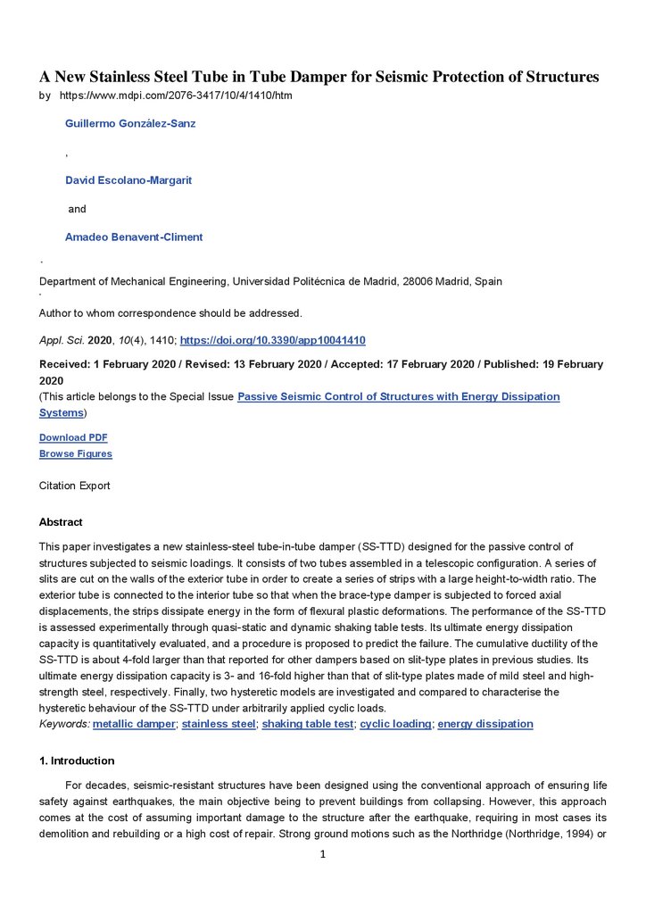
dissipation devices that have drawn attention lately are the slit type (Figure 1a) and the honeycomb damper (Figure
1b). They are built from steel plates with openings of constant width referred to as slits (Figure 1a), or a variable
honeycomb shape (Figure 1b), leaving between them steel strips of constant (Figure 1a) or variable (Figure 1b)
width. These strips dissipate energy through plastic flexural/shear deformations.
Figure 1. Metallic dampers: (a) slit damper; (b) honeycomb damper.
Several recent studies have investigated slit-type dampers made of mild steel. Chan [6] studied a slit damper
fabricated from a standard structural wide-flange section with some slits cut in the web. Teruna [7] investigated
several steel dampers with a honeycomb geometry with the aim of yielding all the length of the strip simultaneously.
Lee [8] proposed several optimized nonuniform shapes for the openings of the damper and compared their overall
performance through quasi-static cyclic tests. Lee [9] developed a series of hourglass-shaped strip dampers and
tested them under quasi-static and dynamic monotonic and cyclic loading. Amiri [10] studied a symmetric slit damper
cut from a steel plate having a low height-to-thickness ratio. The shape and dimensions of several specimens were
optimized and tested experimentally under cyclic loading in quasi-static conditions. Extending the concept of the slittype damper, Benavent [11] devised a tube-in-tube damper based on yielding the walls of hollow mild steel structural
sections, which can be installed in a frame structure as a conventional diagonal brace. Past studies on slit-type
dampers used steel plates made of mild steel, low-yield steel or even high-strength steel [12]. To the knowledge of the
authors, slit-type dampers made of stainless steel have not been reported in the literature.
This study proposes a new Stainless-Steel Tube-in-Tube Damper (hereafter SS-TTD), whose source of energy
dissipation is the plastic deformation of stainless-steel plates with slits. Besides the novelty of using stainless steel
instead of mild or high-strength steel, SS-TTD uses strips with an h/b aspect ratio (see Figure 1a) as large as possible
within the dimensional constraints imposed for architectural reasons (i.e., in conventional buildings, the cross section
of the tubes is limited so that the brace damper can be embedded in partitions or exterior walls). Stainless steel has
an inherent energy dissipation capacity that is markedly larger than that of low-yield steel or mild steel. This is due to
its higher ductility, that is, the amount of plastic deformation that the material can endure until failure [13]. Meanwhile,
largeh/b ratios guarantee a flexural-type yielding mode of the steel strips and enhance the energy dissipation capacity
of the damper. The performance of the SS-TTD in terms of hysteretic behaviour, ductility and ultimate energy
dissipation capacity is investigated through dynamic shaking table tests and quasi-static cyclic tests. A comparison
2

3.

with other metallic dampers proposed in the literature is presented. Finally, two numerical models are proposed and
compared, to predict the hysteretic behaviour and failure of the damper.
2. Proposed Seismic Damper
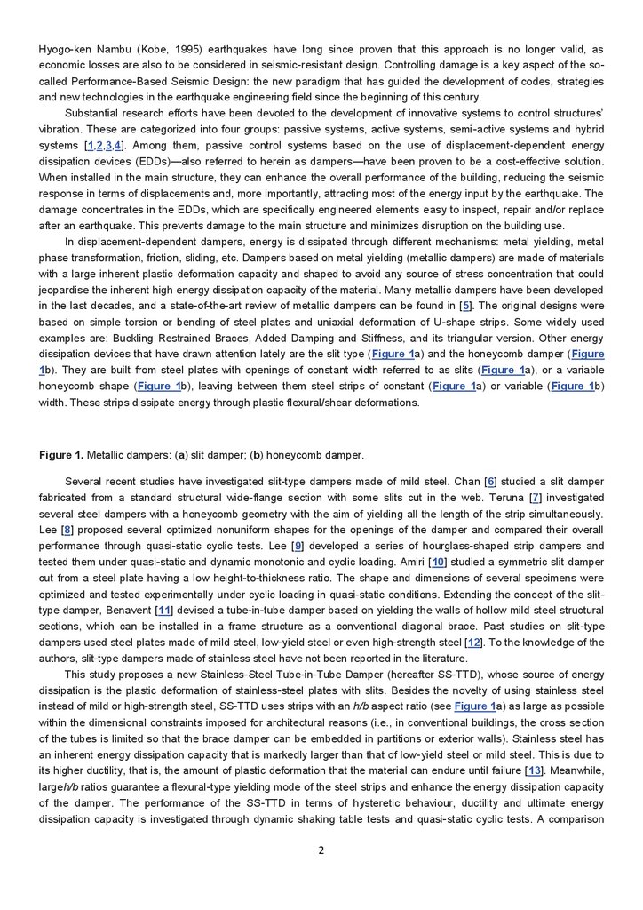
The proposed SS-TTD damper is constructed through the assemblage of two standardized stainless-steel tubes
with a telescopic configuration (Figure 2a). All faces (i.e., the four walls) of the outer tube are regularly slit
transversally to its longitudinal axis, forming strips. The strips are grooved so that one of its sides can be connected to
a common plate, thus linking all in parallel. The common plate that gathers one end of each steel strip is fixed to the
inner tube with plug welding at discrete points. The other end of each steel strip is connected to the corner of the outer
tube. When the brace is subjected to axial forces, the relative displacements between the tubes impose a double
curvature flexural deformation on the strips, which behave as a series of fixed-ended beams. These strips constitute
the energy dissipating part of the SS-TTD. One end of each tube is connected to auxiliary brace members of the
appropriate length that connect the SS-TTD damper to the two points of the building structure that are expected to
undergo large relative horizontal displacements (Figure 2b). Typically, in frame structures, these points are two beamcolumn joints of consecutive spans and floor levels, as shown in Figure 2b.
Figure 2. Proposed damper (a) and installation in a typical building frame (b).
Knowing the geometry and mechanical properties of the stainless steel that form the strips, the axial yielding
forceQy and apparent maximum force QB of the damper are readily obtained by applying fundamental engineering
principles as follows:
Qy=nζytb22h′; QB=nζBtb22h′,
(1)
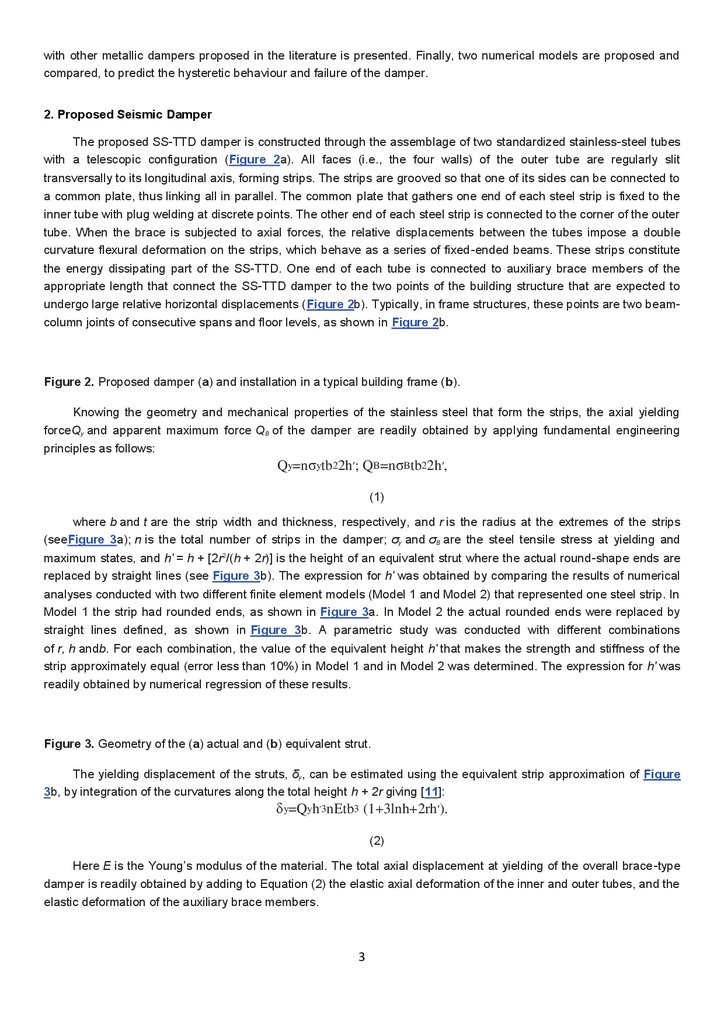
where b and t are the strip width and thickness, respectively, and r is the radius at the extremes of the strips
(seeFigure 3a); n is the total number of strips in the damper; ζy and ζB are the steel tensile stress at yielding and
maximum states, and h′ = h + [2r2/(h + 2r)] is the height of an equivalent strut where the actual round-shape ends are
replaced by straight lines (see Figure 3b). The expression for h′ was obtained by comparing the results of numerical
analyses conducted with two different finite element models (Model 1 and Model 2) that represented one steel strip. In
Model 1 the strip had rounded ends, as shown in Figure 3a. In Model 2 the actual rounded ends were replaced by
straight lines defined, as shown in Figure 3b. A parametric study was conducted with different combinations
of r, h andb. For each combination, the value of the equivalent height h′ that makes the strength and stiffness of the
strip approximately equal (error less than 10%) in Model 1 and in Model 2 was determined. The expression for h′ was
readily obtained by numerical regression of these results.
Figure 3. Geometry of the (a) actual and (b) equivalent strut.
The yielding displacement of the struts, δy, can be estimated using the equivalent strip approximation of Figure
3b, by integration of the curvatures along the total height h + 2r giving [11]:
δy=Qyh′3nEtb3 (1+3lnh+2rh′).
(2)
Here E is the Young’s modulus of the material. The total axial displacement at yielding of the overall brace-type
damper is readily obtained by adding to Equation (2) the elastic axial deformation of the inner and outer tubes, and the
elastic deformation of the auxiliary brace members.
3

4.

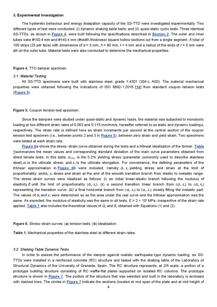
3. Experimental Investigation
The hysteretic behaviour and energy dissipation capacity of the SS-TTD were investigated experimentally. Two
different types of test were conducted: (i) dynamic shaking table tests; and (ii) quasi-static cyclic tests. Three identical
SS-TTDs, as shown in Figure 4, were built following the specifications described in Section 2. The outer and inner
tubes were #150.4 mm and #140.4 mm (#width.thickness) square hollow sections cut from a single segment. A total of
100 strips (25 per face) with dimensions of b = 5 mm, h = 80 mm, t = 4 mm and a radius of the ends of r = 5 mm were
slit on the outer tube. Material tests were also conducted to determine the mechanical properties.
Figure 4. TTD damper specimen.
3.1. Material Testing
All SS-TTD specimens were built with stainless steel, grade 1.4301 (304-L AISI). The material mechanical
properties were obtained following the indications of ISO 6892-1:2016 [14] from standard coupon tension tests
(Figure 5).
Figure 5. Coupon tension test specimen.
Since the dampers were studied under quasi-static and dynamic loads, the material was subjected to monotonic
loading at two different strain rates of 0.003 and 0.115 mm/mm/s, hereafter referred to as static and dynamic loadings,
respectively. The strain rate is defined here as strain increments per second at the central section of the coupon
tension test specimen (i.e., between points 2 and 3 in Figure 5), between zero strain and yield strain. Two specimens
were tested at each strain rate.
Figure 6a shows the stress‒strain curve obtained during the tests and a trilineal idealisation of the former. Table
1summarizes the mean values and corresponding standard deviation of the main curve parameters obtained from
direct tensile tests. In this table, ζ0.2%, is the 0.2% yielding stress (parameter commonly used to describe stainless
steel),ζu is the ultimate stress, and εu is the ultimate elongation. For convenience, the defining parameters of the
trilinear approximation in Figure 6b were included, namely: ζy, εy yielding stress and strain at the limit of
proportionality; andζb, εb stress and strain at the end of the smooth transition branch from elastic to inelastic range.
The stress‒strain curves were idealized as follows: (i) an initial linear-elastic branch following the modulus of
elasticity E until the limit of proportionality (ζy, εy); (ii) a second transition linear branch from (ζy, εy) to (ζb, εb)
representing the transition curve; (iii) a final horizontal branch from (ζb, εb) to (ζu, εu) closely fitting the inelastic part.
The values of ζb and εb were determined so as the area under the real curve and the trilinear approximation was the
same. As expected, the modulus of elasticity was the same in all tests, E = 2 × 105 MPa, irrespective of the strain rate
applied. Table 1 also includes the theoretical values of Qy and δy obtained with Equations (1) and (2).
Figure 6. Stress‒strain curves: (a) tension tests; (b) idealisation.
Table 1. Mechanical properties of the stainless steel at different strain rates.
3.2. Shaking Table Dynamic Tests
In order to assess the performance of the damper against realistic earthquake-type dynamic loading, six SSTTDs were installed in a reinforced concrete (RC) structure and tested with the shaking table of the Laboratory of
Structural Dynamics of the University of Granada, Spain. The RC structure represents, at 2/5 scale, a portion of a
prototype building structure consisting of RC waffle-flat plates supported on isolated RC columns. The prototype
structure is shown in Figure 7. The portion of the structure that was selected and built in the laboratory is enclosed
with dashed lines. The circles in Figure 7 indicate the sections (located at mid span of the plate and at mid height of
4

5.

the columns) where the bending moment is assumed to be zero under horizontal loads. The prototype structure was
designed to sustain gravity loads only, according to the Spanish construction codes [15,16]. Figure 8 shows the
portion of the prototype RC structure with the SS-TTDs mounted on the shaking table. As seen in Figure 8, three SSTTDs were installed in each storey as diagonal bars. The three identical SS-TTDs shown in Figure 4 were installed in
the upper storey, and will be referred to as SS-TTD4, SS-TTD5 and SS-TTD6. Reactive steel blocks were located at
the top columns and on the waffle-flat plate to reproduce the mass of the upper part of the structure and to satisfy
similitude laws. Figure 9 shows the overall experimental set-up. A detailed description of a similar reinforced structure
tested by the authors in previous studies and with a different type of damper can be found in [17].
Figure 7. Sketch of the whole structure.
Figure 8. RC structure with SS-TTDs. (a) View in plan and (b) in elevation.
Figure 9. General overview of the experimental setup used for the shaking table tests.
The seismic tests were performed with a bidirectional MTS 3 × 3 m2 shaking table. The setup of instrumentation
included uniaxial accelerometers, displacement transducers (LVDTs) and more than 400 strain gauges set in the
whole structure. On the SS-TTDs, a pair of LVDTs for each damper measured the mean values of the relative axial
displacements between the tubes. Axial forces were obtained as the average value from six strain gauges fixed to the
auxiliary square hollow sections (#80.4 mm) connecting the SS-TTD to the main structure. Figure 8 shows the test
specimen equipped with the SS-TTDs and the setup and instrumentation utilized.
The RC structure with the SS-TTDs was subjected to eight seismic simulations. In all simulations the two
horizontal components, north‒south (NS) and east‒west (EW), of ground motion acceleration recorded at BarSkupstina Opstine during the Montenegro earthquake (1979) were simultaneously applied, scaled in amplitude by a
factor that was successively increased from 15% of the original record to 190%. The NS component was applied in
the direction of the axis of symmetry of the test specimen (referred to as direction X), and the EW component in the
orthogonal direction (referred to as direction Y). Figure 10 shows the histories of acceleration applied to the shaking
table in the X and Y horizontal directions. Figure 11 shows the movements of the reactive steel blocks located at the
top of the columns of the upper storey; more precisely, the relative displacements in the X and Y horizontal directions
with respect to the RC waffle-flat plate, and the rotations about the vertical axis passing through the centre of mass. It
can be seen that the relative displacements in the Y direction (Figure 11b) are about two times larger than in the X
direction (Figure 11a). The corresponding maximum inter storey drifts (i.e., the relative displacement divided by the
height of the columns) were about 1% in the X direction and 2% in the Y direction. These values are below the limit of
2.5% associated with the performance level of life safety, and far below the 4% associated with collapse in previous
studies on RC waffle-flat plate systems [17]. This means that the SS-TTDs protected the structure against collapse
and kept it within reasonable levels of safety when subjected to ground motions with peak ground accelerations as
large as 1g (here g is the acceleration of gravity), as shown in Figure 10.
Figure 10. History of accelerations applied to the shaking table.
5

6.

Figure 11. History of displacements and rotations of the reactive steel blocks located at the top of the columns of the
upper storey during the shaking table tests: relative displacement in the X (a) and Y (b) horizontal directions, and
rotation (c) about the axis passing through its centre of mass.
In the 1st, 2nd and 3rd seismic simulations the SS-TTDs remained elastic with maximum axial displacements of
0.2δyDYN, 0.5δyDYN and 0.9δyDYN. During the following seismic simulations, the SS-TTDs underwent plastic deformations
and reached maximum axial displacements of up to 5.2δyDYN. This study focuses on the results obtained from the SSTTDs located on the upper floor, namely SS-TTD4, SS-TTD5, and SS-TTD6. The overall response in terms of axial
force vs. axial displacement of these SS-TTDs can be seen in Figure 12. At the end of the seismic simulations, the
main RC structure (columns and waffle-flat slab) remained basically elastic (i.e., with no damage); the steel
reinforcement did not experience any plastic deformation and only minor cracking was observed in the concrete. In
contrast, the SS-TTD endured large plastic deformations but without failure, i.e., the SS-TTDs did not reach their
ultimate energy dissipation capacity.
Figure 12. Q‒δ curves obtained from the shaking table tests: (a) SS-TTD4, (b) SS-TTD5, (c) SS-TTD6.
3.3. Quasi-Static Cyclic Tests
After performing the shaking table dynamic tests, the SS-TTDs installed in the upper storey were subjected to
cyclic quasi-static loading until failure in order to quantify their ultimate energy dissipation capacity. The specimens
were disassembled from the RC structure and tested on a SAXEWAY T1000 universal testing machine with a
maximum load capacity of 1000 kN, as shown in Figure 13. Both the inner and outer tube were welded to a 25-mm
base plate that was rigidly bolted to the base of the testing machine and to the actuator, respectively. All the tests
were carried out under displacement control with the same cyclic rate of 0.02 Hz. Two displacement transducers
(LVDTs), connecting the inner and outer tubes in the direction of the applied load, controlled and measured relative
displacements between the tubes. Three different loading histories consisting of cyclic forced displacements were
applied to the SS-TTDs. Specimen SS-TTD4 was subjected to an initial displacement of 10 mm in the positive
direction followed by cycles of constant amplitude equal to 5 times the yield displacement δyST. Specimens SS-TTD5
and SS-TTD6 were subjected to sequential sets of cycles with incremental amplitude, following the protocol proposed
by ATC [18]. In both cases the increment of displacement amplitude from one set of cycles to the next, Δδ, was
Δδ/δYst = 1; the difference was the number of cycles nc applied within each set. For specimen SS-TTD5 nc = 10, while
for specimen SS-TTD6 nc = 4. The SS-TTD damper was assumed to fail when the force under increasing
displacements dropped below 20% of the maximum force attained in previous cycles of deformation.
Figure 13. Experimental setup for static cyclic tests: (a) identification of components, (b) photograph.
The entire axial force‒displacement, Q‒δ, hysteretic curves obtained from the quasi-static cyclic tests are plotted
in dotted lines in Figure 14. The solid line represents the hysteretic behaviour before failure, with the dotted lines
showing the Q‒δ curves after failure.
Figure 14. Q‒δ curves obtained from the quasi-static cyclic tests: (a) SS-TTD4, (b) SS-TTD5, (c) SS-TTD6.
4. Results and Discussion
4.1. Hysteretic Behaviour
The seismic performance of the SS-TTDs is readily characterised in the complete loaddisplacement Q‒δhysteretic curves of Figure 15; it combines the curves obtained from the shaking table tests and
from the quasi-static tests. Since the yield force and yield displacement are different under quasi-static (i.e., QyST =
6

7.

15.5 kN, δyST = 1.08 mm), and under dynamic loads (i.e., QyDYN = 24.83 kN, δyDYN = 1.73 mm) due to strain rate effects
[19,20,21], prior to combining the Q‒δ curves they were normalized by the corresponding yielding force and yielding
displacement. From the Q‒δ curves shown in Figure 15 the following observations can be made. First, the SS-TTD
exhibits a stable hysteretic behaviour. Second, the Q‒δ curves under repeated cycles of the same amplitude are
almost coincident, that is, the reduction of the peak strength under repeated cycles of constant amplitude is small.
Third, second order effects due to strip geometric nonlinearity appear when the imposed displacements are very large,
more precisely at displacement ductility µ = δmax/δyST above 12. This geometric nonlinearity results in a spurious
increase of the restoring force. It must be noted, however, that the value of the ductility µ (i.e., about 12) beyond which
the geometric nonlinearity effects become significant is far beyond the realistic range of lateral displacements that
could be allowed in actual structures equipped with dampers. More precisely, in flexible RC frames or RC waffle-flat
plate systems, damage starts for interstorey drifts, ID, between 0.005 and 0.01 times the storey height H [17,22]. Even
if some (moderate) damage is allowed in the RC structure to reduce the cost of the dampers, the ID should not
exceed about 0.015H, because otherwise installing the dampers would be meaningless. Assuming a realistic storey
height (after scaling by the scaling factor of the test specimen 2/5) of H = 3000 × 2/5 = 1200 mm, and an angle of the
SS-TTD axis with the horizontal α = 0.46 rad, the maximum axial displacement δmax (=H × ID × cosα) normalized by the
yield displacementδyDYN (=1.73 mm), i.e., δmax/δyDYN, to be allowed in the SS-TTD to prevent damage in the main RC
structure would range between 3.1 and 6.2, and should be smaller than 9.3 in any case. These values are below the
axial displacement ductility μ (= 12) corresponding to the onset of the second order effects.
Figure 15. Total normalized Q‒δ curves of the tested specimens: (a) SS-TTD4, (b) SS-TTD5, (c) SS-TTD6.
The shape of the hysteretic loop Q‒δ obtained in one cycle of imposed deformation at maximum amplitude δmax is
typically characterised by the equivalent viscous ratio ξ, defined as follows:
ξ=12πWcQmaxδmax,
(3)
where Wc is the energy dissipated in one cycle and Qmax the force attained at δmax. This formula is obtained by
equating the hysteretic energy dissipated in one cycle and the energy dissipated through viscous damping by means
of an equivalent viscous damper in one cycle of harmonic vibration [23]. The larger ξ is, the closer the shape of the
hysteretic loop to an ideal parallelogram. ξ was calculated for the hysteretic loops obtained from the SS-TTDs
subjected to cycles of incremental amplitude; the results are displayed in Figure 16 against the amplitude of the
cycle δmaxnormalized by δy. It can be seen that for practical values of δmax/δy (between approximately 6.2 and 9.3), the
equivalent viscous damping ξ remains approximately constant at 30%. This value is compared in the last column
of Table 2 with the ξ’s obtained in previous studies [6,7,8,10] for slit-type plates with different geometries
(h, b, t shown in Figure 3) and material properties of the steel (ζY). It can be seen that the value of ξ for the damper
proposed in this study is within the range (30%–51%) found for other types of dampers in previous studies, although in
the lower bound. This means that the proposed damper does not present advantages in comparison to other dampers
from the point of view of the amount of energy that can be dissipated per cycle for fixed values of Qmax and δmax. Table
2 also shows the accumulated inelastic deformation ratio, η, and the cumulative ductility factor [6,7,8,9,10,11], μCUM,
that are typical parameters used to characterise the performance of dampers. These parameters are defined later in
Equations (5) and (7), respectively.
Figure 16. Equivalent viscous damping ξ versus the normalized cycle amplitude.
Table 2. Comparison with other slit-type steel plate dampers.
4.2. Ultimate Energy Dissipation Capacity and Prediction of Failure
7

8.

Previous studies [24,25,26] have pointed out the dependence of the ultimate energy dissipation capacity of
structural members subjected to low-cycle fatigue on the pattern of loading applied. An appropriate way [24,25] to take
into account this dependency consists of splitting the total energy dissipated by the damper into two parts: the energy
dissipated on the so-called skeleton part and the energy dissipated on the Bauschinger part, as shown in Figure 17.
The typical Q‒δ curve obtained by testing a steel component under arbitrarily applied cyclic loads until failure (Figure
17a) can be decomposed into the skeleton part (Figure 17b) and Bauschinger part (Figure 17c) as follows. The
skeleton part is formed, in each domain of loading, by connecting sequentially the segments of the Q‒δ curve whose
force Q exceeds the maximum force attained in previous cycles in the same domain of loading. The skeleton curves
obtained in this way coincide with the Q‒δ obtained by subjecting the steel component to monotonic loadings [25].
The skeleton curves are idealized by the trilinear curve in Figure 17b (dashed and dotted lines), in turn defined by the
following parameters: Qy and δy given by Equations (1) and (2); the elastic stiffness Ke (=Qy /δy); the force QB at the
onset of the second plastic branch given by Equation (1); and the first and second plastic stiffness, Kp1 and Kp2. The
displacement δB associated with QB is readily obtained from Kp1 and QB. In Figure 17b, Sδu+ and Sδu− denote the
maximum deformation accumulated in the positive and negative skeleton parts. The portion of the total plastic strain
energy dissipated by the damper on the skeleton part, in the positive and negative domains of loading,
respectivelySWu+ and SWu−, is readily obtained by integrating the areas enveloped by each skeleton curve in Figure
17b. The Bauschinger part is constituted by the segments of the Q‒δ curve that start at Q = 0 and end at the point
corresponding to the maximum load attained in the preceding cycles in the same loading domain. The Bauschinger
parts are graphically depicted in Figure 17c, and the area enveloped in each domain of loading, BWu+ and BWu−,
represents the portion of the total energy dissipated by the steel element in the Bauschinger part.
Figure 17. Decomposition of Q‒δ curve: (a) overall curve; (b) skeleton part; (c) Bauschinger part.
For convenience, SWu+, SWu−, BWu+, BWu−, Sδu+ and Sδu−, are expressed in a nondimensional form by:
Sη¯+=SW+uQyδy;η¯S−=SW−uQyδy;η¯B+=BW+uQyδ y;η¯B−=BW−uQyδy;η¯ep+=Sδ+uδy;η¯ep−=Sδ−uδy
(4)
and the total energy dissipated on the skeleton part, on the Bauschinger part, and the total energy dissipated by
the steel component until failure can be expressed in nondimensional form by:
ηS=∣∣η¯S+∣∣+∣∣η¯S−∣∣;ηB=∣∣η¯B+∣∣+∣∣η¯B−∣∣;ηep=∣∣η¯ep+∣∣+∣∣η¯ep−∣∣;η=ηS+ηB.
(5)
Past studies [12] showed that ηB and ηep follow an approximately linear relationship:
ηB=aηep+b′,
(6)
where a and b′ are two parameters determined from tests.
The normalized Q‒δ curves obtained in each test until failure (Figure 15) were decomposed as explained above
and the values obtained for the nondimensional parameters defined in Equations (4) and (5) are summarized in Table
3.Figure 18 shows the normalized skeleton curves together with an approximated trilinear curve (bold dotted line)
wherekp1 = 1/2.5 and kp2 = 1/14. Figure 19a–c shows with circle, rhombus and square symbols the values
of Sη, Bη and ηat failure obtained from the tested specimens; they are plotted against epη. The decomposition explained
above was also done at each point of the normalized Q‒δ curves of Figure 15, the corresponding values of Sη, Bη,
η and epη are plotted with solid lines in Figure 19. These curves represent the ―energy dissipation path‖ followed by
each test specimen up to failure. Also plotted in Figure 19a is a line (solid bold) with slope a = −14.66 passing through
the point (0, 3900), which is found to fit the experimental results well. This value a = −14.66 is the one obtained in
previous studies [12] for slit-type plates made of mild and high-strength steel; thus the results of this study indicate it is
likewise valid for the slit-type plates made of stainless steel. As for parameter b′, from the experimental results of this
8

9.

study it is proposed to adopt b′ = 3900 for slit-type plates made of stainless steel. The value of parameter b′ is a good
indicator of the ultimate energy dissipation capacity of the damper. Comparing the b′ obtained for the new SS-TTD
damper—b′ = 3900—with that reported in previous studies on slit-plates made of mild steel [12] and high-strength
steel [12]—b′ = 1325 and b′ = 250, respectively—it is concluded that the ultimate energy dissipation capacity of the
stainless-steel slit-type plates that form the new SS-TTD is about three times larger than that of the mild steel slit-type
plates, and 16 times larger than that of the high-strength steel slit-type plates.
Figure 18. Skeleton curves.
Figure 19. Ultimate energy dissipation capacity: (a) Bauschinger part, (b) skeleton part, (c) total.
Table 3. Ultimate energy dissipation capacity.
The solid bold line in Figure 19b represents the normalized energy dissipated on the skeleton part against epη. It
was calculated using the approximated trilinear skeleton curve shown in Figure 18 with dotted bold lines. It is found to
fit the experimental results very well (i.e., circle, rhombus and square symbols). Finally, the solid bold lines of Figure
19a,b were redrawn in Figure 19c (thin solid line and thin dotted line) and summed up to obtain the solid bold line
ofFigure 19c that represents the normalized ultimate energy dissipation capacity of the SS-TTD, characterised by
parameters kp1 = 1/2.5, kp2 = 1/14, a = −14.66, b = 3900 and the values of Qy, QB, δy given by Equations (1) and (2).
Once the ultimate energy dissipation capacity of the SS-TTD is determined, the failure of the SS-TTD under arbitrarily
applied cyclic loading can be predicted from the Q‒δ curve obtained up to each instant from numerical simulations
(i.e., nonlinear time history analysis) as follows. At any instant i, the values of epη and η are calculated from
the Q‒δ curve obtained up to instant i as explained above, they are named epηi and ηi hereafter. Tracking this pair of
points (epηi, ηi) and plotting them in Figure 19c, failure is expected to occur when the solid bold line is reached.
Previous studies [6,7,8,9,10,11] related the ultimate energy dissipation capacity of the damper to the cumulative
ductility factor μCUM defined by Equation (7). In this equation, ∑δ is the sum of excursions of displacement experienced
by the damper, normalized by the yielding displacement δy. Figure 20 shows the normalized ultimate energy
dissipation capacity η against μCUM obtained for the SS-TTDs tested in this study until failure.
μCUM=∑δδy
(7)
Figure 20. Normalized ultimate energy dissipation capacity against cumulative ductility factor.
The pair of values (η, μCUM) at failure obtained for the SS-TTDs are plotted in Figure 21 and compared with the
values obtained in previous studies [6,7,8,9]. It is seen that the proposed SS-TTD has an energy dissipation capacity
and an accumulated ductility notably larger than those reported for other dampers in previous studies.
Figure 21. Comparison of the η‒μCUM relationship between the selected references and this study.
5. Numerical Characterization
9

10.

Two different numerical models were investigated to predict the hysteretic behaviour of the SS-TTD under
arbitrary cyclic loadings. The first one is the polygonal model based on piecewise linear segments. The second one is
a smooth hysteretic Bouc‒Wen model [27], characterised by a continuous change of stiffness due to yielding and
sharp changes from loading to unloading paths.
5.1. Polygonal Model
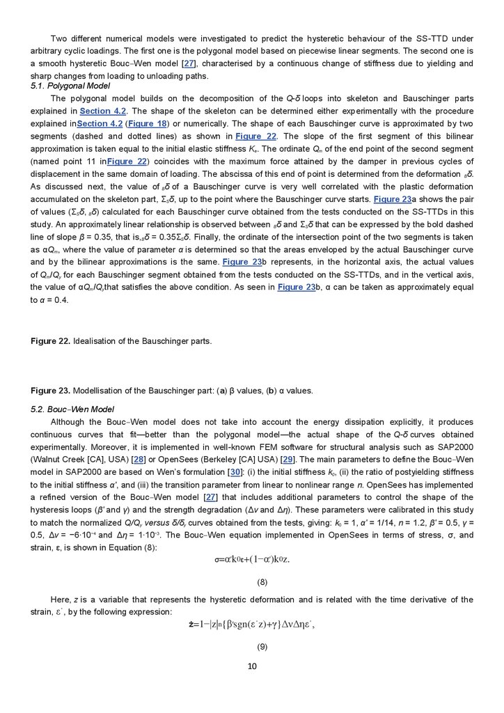
The polygonal model builds on the decomposition of the Q-δ loops into skeleton and Bauschinger parts
explained in Section 4.2. The shape of the skeleton can be determined either experimentally with the procedure
explained inSection 4.2 (Figure 18) or numerically. The shape of each Bauschinger curve is approximated by two
segments (dashed and dotted lines) as shown in Figure 22. The slope of the first segment of this bilinear
approximation is taken equal to the initial elastic stiffness Ke. The ordinate Qm of the end point of the second segment
(named point 11 inFigure 22) coincides with the maximum force attained by the damper in previous cycles of
displacement in the same domain of loading. The abscissa of this end of point is determined from the deformation Bδ.
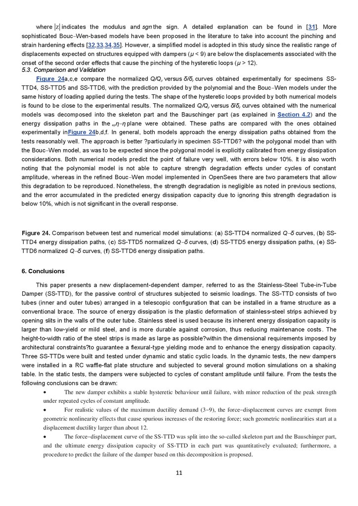
As discussed next, the value of Bδ of a Bauschinger curve is very well correlated with the plastic deformation
accumulated on the skeleton part, ΣSδ, up to the point where the Bauschinger curve starts. Figure 23a shows the pair
of values (ΣSδ, Bδ) calculated for each Bauschinger curve obtained from the tests conducted on the SS-TTDs in this
study. An approximately linear relationship is observed between Bδ and ΣSδ that can be expressed by the bold dashed
line of slope β = 0.35, that is,Bδ = 0.35ΣSδ. Finally, the ordinate of the intersection point of the two segments is taken
as αQm, where the value of parameter α is determined so that the areas enveloped by the actual Bauschinger curve
and by the bilinear approximations is the same. Figure 23b represents, in the horizontal axis, the actual values
of Qm/Qy for each Bauschinger segment obtained from the tests conducted on the SS-TTDs, and in the vertical axis,
the value of αQm/Qythat satisfies the above condition. As seen in Figure 23b, α can be taken as approximately equal
to α = 0.4.
Figure 22. Idealisation of the Bauschinger parts.
Figure 23. Modellisation of the Bauschinger part: (a) β values, (b) α values.
5.2. Bouc‒Wen Model
Although the Bouc‒Wen model does not take into account the energy dissipation explicitly, it produces
continuous curves that fit—better than the polygonal model—the actual shape of the Q-δ curves obtained
experimentally. Moreover, it is implemented in well-known FEM software for structural analysis such as SAP2000
(Walnut Creek [CA], USA) [28] or OpenSees (Berkeley [CA] USA) [29]. The main parameters to define the Bouc‒Wen
model in SAP2000 are based on Wen’s formulation [30]: (i) the initial stiffness k0, (ii) the ratio of postyielding stiffness
to the initial stiffness α′, and (iii) the transition parameter from linear to nonlinear range n. OpenSees has implemented
a refined version of the Bouc‒Wen model [27] that includes additional parameters to control the shape of the
hysteresis loops (β′ and γ) and the strength degradation (Δν and Δη). These parameters were calibrated in this study
to match the normalized Q/Qy versus δ/δy curves obtained from the tests, giving: k0 = 1, α′ = 1/14, n = 1.2, β′ = 0.5, γ =
0.5, Δν = −6·10−4 and Δη = 1·10−3. The Bouc‒Wen equation implemented in OpenSees in terms of stress, σ, and
strain, ε, is shown in Equation (8):
σ=α′k0ε+(1−α′)k0z.
(8)
Here, z is a variable that represents the hysteretic deformation and is related with the time derivative of the
strain, ε˙, by the following expression:
ż=1−|z|n{β′sgn(ε˙z)+γ}ΔνΔηε˙,
(9)
10

11.

where
|z| indicates the modulus and sgn the sign. A detailed explanation can be found in [31]. More
sophisticated Bouc‒Wen-based models have been proposed in the literature to take into account the pinching and
strain hardening effects [32,33,34,35]. However, a simplified model is adopted in this study since the realistic range of
displacements expected on structures equipped with dampers (μ < 9) are below the displacements associated with the
onset of the second order effects that cause the pinching of the hysteretic loops (μ > 12).
5.3. Comparison and Validation
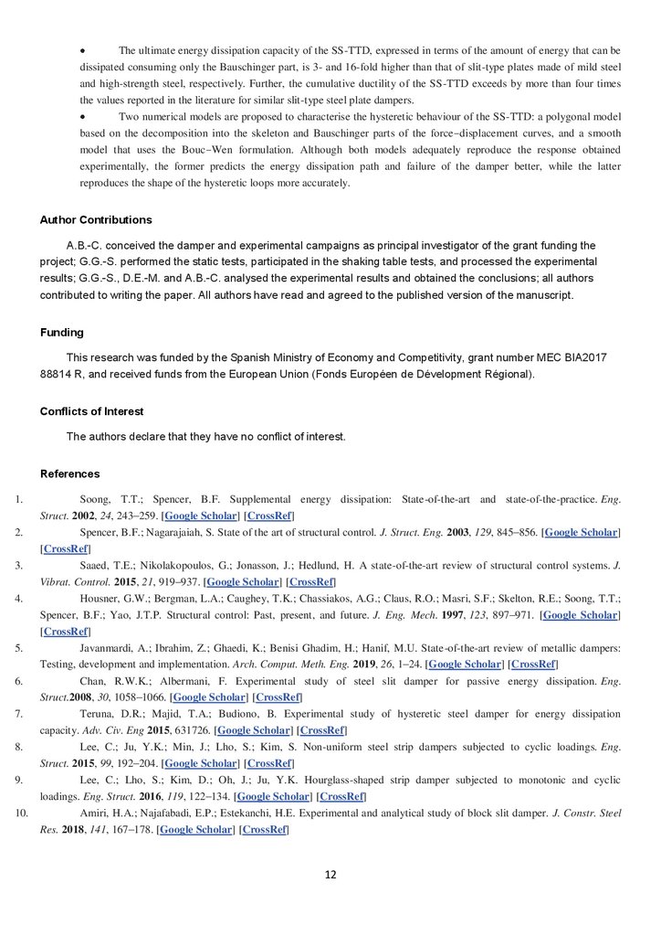
Figure 24a,c,e compare the normalized Q/Qy versus δ/δy curves obtained experimentally for specimens SSTTD4, SS-TTD5 and SS-TTD6, with the prediction provided by the polynomial and the Bouc‒Wen models under the
same history of loading applied during the tests. The shape of the hysteretic loops provided by both numerical models
is found to be close to the experimental results. The normalized Q/Qy versus δ/δy curves obtained with the numerical
models was decomposed into the skeleton part and the Bauschinger part (as explained in Section 4.2) and the
energy dissipation paths in the epη‒η plane were obtained. These paths are compared with the ones obtained
experimentally inFigure 24b,d,f. In general, both models approach the energy dissipation paths obtained from the
tests reasonably well. The approach is better ?particularly in specimen SS-TTD6? with the polygonal model than with
the Bouc‒Wen model, as was to be expected since the polygonal model is explicitly calibrated from energy dissipation
considerations. Both numerical models predict the point of failure very well, with errors below 10%. It is also worth
noting that the polynomial model is not able to capture strength degradation effects under cycles of constant
amplitude, whereas in the refined Bouc‒Wen model implemented in OpenSees there are two parameters that allow
this degradation to be reproduced. Nonetheless, the strength degradation is negligible as noted in previous sections,
and the error accumulated in the predicted energy dissipation capacity due to ignoring this strength degradation is
below 10%, which is not significant in the overall response.
Figure 24. Comparison between test and numerical model simulations: (a) SS-TTD4 normalized Q‒δ curves, (b) SSTTD4 energy dissipation paths, (c) SS-TTD5 normalized Q‒δ curves, (d) SS-TTD5 energy dissipation paths, (e) SSTTD6 normalized Q‒δ curves, (f) SS-TTD6 energy dissipation paths.
6. Conclusions
This paper presents a new displacement-dependent damper, referred to as the Stainless-Steel Tube-in-Tube
Damper (SS-TTD), for the passive control of structures subjected to seismic loadings. The SS-TTD consists of two
tubes (inner and outer tubes) arranged in a telescopic configuration that can be installed in a frame structure as a
conventional brace. The source of energy dissipation is the plastic deformation of stainless-steel strips achieved by
opening slits in the walls of the outer tube. Stainless steel is used because its inherent energy dissipation capacity is
larger than low-yield or mild steel, and is more durable against corrosion, thus reducing maintenance costs. The
height-to-width ratio of the steel strips is made as large as possible?within the dimensional requirements imposed by
architectural constraints?to guarantee a flexural-type yielding mode and to enhance the energy dissipation capacity.
Three SS-TTDs were built and tested under dynamic and static cyclic loads. In the dynamic tests, the new dampers
were installed in a RC waffle-flat plate structure and subjected to several ground motion simulations on a shaking
table. In the static tests, the dampers were subjected to cycles of constant amplitude until failure. From the tests the
following conclusions can be drawn:
The new damper exhibits a stable hysteretic behaviour until failure, with minor reduction of the peak strength
under repeated cycles of constant amplitude.
For realistic values of the maximum ductility demand (3‒9), the force‒displacement curves are exempt from
geometric nonlinearity effects that cause spurious increases of the restoring force; such geometric nonlinearities start at a
displacement ductility larger than about 12.
The force‒displacement curve of the SS-TTD was split into the so-called skeleton part and the Bauschinger part,
and the ultimate energy dissipation capacity of SS-TTD in each part was quantitatively evaluated; furthermore, a
procedure to predict the failure of the damper based on this decomposition is proposed.
11

12.

The ultimate energy dissipation capacity of the SS-TTD, expressed in terms of the amount of energy that can be
dissipated consuming only the Bauschinger part, is 3- and 16-fold higher than that of slit-type plates made of mild steel
and high-strength steel, respectively. Further, the cumulative ductility of the SS-TTD exceeds by more than four times
the values reported in the literature for similar slit-type steel plate dampers.
Two numerical models are proposed to characterise the hysteretic behaviour of the SS-TTD: a polygonal model
based on the decomposition into the skeleton and Bauschinger parts of the force‒displacement curves, and a smooth
model that uses the Bouc‒Wen formulation. Although both models adequately reproduce the response obtained
experimentally, the former predicts the energy dissipation path and failure of the damper better, while the latter
reproduces the shape of the hysteretic loops more accurately.
Author Contributions
A.B.-C. conceived the damper and experimental campaigns as principal investigator of the grant funding the
project; G.G.-S. performed the static tests, participated in the shaking table tests, and processed the experimental
results; G.G.-S., D.E.-M. and A.B.-C. analysed the experimental results and obtained the conclusions; all authors
contributed to writing the paper. All authors have read and agreed to the published version of the manuscript.
Funding
This research was funded by the Spanish Ministry of Economy and Competitivity, grant number MEC BIA2017
88814 R, and received funds from the European Union (Fonds Européen de Dévelopment Régional).
Conflicts of Interest
The authors declare that they have no conflict of interest.
References
1.
2.
3.
4.
5.
6.
7.
8.
9.
10.
Soong, T.T.; Spencer, B.F. Supplemental energy dissipation: State-of-the-art and state-of-the-practice. Eng.
Struct. 2002, 24, 243–259. [Google Scholar] [CrossRef]
Spencer, B.F.; Nagarajaiah, S. State of the art of structural control. J. Struct. Eng. 2003, 129, 845–856. [Google Scholar]
[CrossRef]
Saaed, T.E.; Nikolakopoulos, G.; Jonasson, J.; Hedlund, H. A state-of-the-art review of structural control systems. J.
Vibrat. Control. 2015, 21, 919–937. [Google Scholar] [CrossRef]
Housner, G.W.; Bergman, L.A.; Caughey, T.K.; Chassiakos, A.G.; Claus, R.O.; Masri, S.F.; Skelton, R.E.; Soong, T.T.;
Spencer, B.F.; Yao, J.T.P. Structural control: Past, present, and future. J. Eng. Mech. 1997, 123, 897–971. [Google Scholar]
[CrossRef]
Javanmardi, A.; Ibrahim, Z.; Ghaedi, K.; Benisi Ghadim, H.; Hanif, M.U. State-of-the-art review of metallic dampers:
Testing, development and implementation. Arch. Comput. Meth. Eng. 2019, 26, 1–24. [Google Scholar] [CrossRef]
Chan, R.W.K.; Albermani, F. Experimental study of steel slit damper for passive energy dissipation. Eng.
Struct.2008, 30, 1058–1066. [Google Scholar] [CrossRef]
Teruna, D.R.; Majid, T.A.; Budiono, B. Experimental study of hysteretic steel damper for energy dissipation
capacity. Adv. Civ. Eng 2015, 631726. [Google Scholar] [CrossRef]
Lee, C.; Ju, Y.K.; Min, J.; Lho, S.; Kim, S. Non-uniform steel strip dampers subjected to cyclic loadings. Eng.
Struct. 2015, 99, 192–204. [Google Scholar] [CrossRef]
Lee, C.; Lho, S.; Kim, D.; Oh, J.; Ju, Y.K. Hourglass-shaped strip damper subjected to monotonic and cyclic
loadings. Eng. Struct. 2016, 119, 122–134. [Google Scholar] [CrossRef]
Amiri, H.A.; Najafabadi, E.P.; Estekanchi, H.E. Experimental and analytical study of block slit damper. J. Constr. Steel
Res. 2018, 141, 167–178. [Google Scholar] [CrossRef]
12

13.

11.
12.
13.
14.
15.
16.
17.
18.
19.
20.
21.
22.
23.
24.
25.
26.
27.
28.
29.
30.
31.
32.
33.
Benavent-Climent, A. A brace-type seismic damper based on yielding the walls of hollow structural sections.Eng.
Struct. 2010, 32, 1113–1122. [Google Scholar] [CrossRef]
Benavent-Climent, A.; Oh, S.; Akiyama, H. Ultimate energy absorption capacity of slit-type steel plates subjected to
shear deformations. J. Struct. Constr. Eng. 1998, 503, 139–147. [Google Scholar] [CrossRef]
Nip, K.H.; Gardner, L.; Elghazouli, A.Y. Cyclic testing and numerical modelling of carbon steel and stainless steel
tubular bracing members. Eng. Struct. 2010, 32, 424–441. [Google Scholar] [CrossRef]
The International Organization for Standardization (ISO). Metallic Materials. Tensile Testing. Part 1: Method of Test at
Room Temperature; UNE-EN ISO 6892-1:2016; The International Organization for Standardization (ISO): Madrid, Spain, 2017.
[Google Scholar]
Ministerio de Fomento. Instrucción de Hormigón Estructural. In Estructuras de Hormigón estructural (EHE-08); Centro
Publicaciones: Madrid, Spain, 2008. [Google Scholar]
Ministerio de Fomento. Norma de Construcción Sismorresistente. In Parte General y Edificación (NSCE-02); Centro
Publicaciones: Madrid, Spain, 2003. [Google Scholar]
Benavent-Climent, A.; Gale-Lamuela, D.; Donaire-Avila, J. Energy capacity and seismic performance of RC waffle-flat
plate structures under two components of far-field ground motions: Shake table tests. Earthq. Eng. Struct. Dyn. 2019, 48, 949–
969. [Google Scholar] [CrossRef]
ATC. Guidelines for Cyclic Seismic Testing of Components of Steel Structures; Applied Technology Council: Redwood
City, CA, USA, 1992. [Google Scholar]
Cadoni, E.; Fenu, L.; Forni, D. Strain rate behaviour in tension of austenitic stainless steel used for reinforcing
bars. Constr. Build. Mater. 2012, 35, 399–407. [Google Scholar] [CrossRef]
Lichtenfeld, J.A.; Mataya, M.C.; Van Tyne, C.J. Effect of strain rate on stress-strain behavior of alloy 309 and 304L
austenitic stainless steel. Metall. Mater. Trans. 2006, 37, 147–161. [Google Scholar] [CrossRef]
Lee, W.S.; Lin, C.F.; Chen, B.T. Tensile properties and microstructural aspects of 304L stainless steel weldments as a
function of strain rate and temperature. Proc. Inst. Mech. Eng. Part C-J. Eng. Mech. Eng. Sci.2005, 219, 439–451. [Google
Scholar] [CrossRef]
Benavent-Climent, A.; Donaire-Avila, J.; Oliver-Saiz, E. Shaking table tests of a reinforced concrete waffle–flat plate
structure designed following modern codes: Seismic performance and damage evaluation. Earthq. Eng. Struct. Dyn. 2016, 45,
315–336. [Google Scholar] [CrossRef]
Chopra, A.K. Dynamics of Structures; Prentice Hall: Englewood Cliffs, NJ, USA, 1995; Volume 3. [Google Scholar]
Benavent-Climent, A. An energy-based damage model for seismic response of steel structures. Earthq. Eng. Struct.
Dyn. 2007, 36, 1049–1064. [Google Scholar] [CrossRef]
Kato, B.; Akiyama, H.; Yamanouchi, H. Predictable Properties of Structural Steels Subjected to Incremental Cyclic
Loading. In IABSE Symposium on Resistance and Ultimate Deformability of Structures Acted on by Well-Defined Loads; IABSEAIPC-IVBH Publications: Lisbon, Portugal, 1973; pp. 119–124. [Google Scholar]
Jiao, Y.; Shimada, Y.; Kishiki, S.; Yamada, S. Study of Energy Dissipation Capacity of Steel Beams Under Cyclic
Loading. In Behaviour of Steel Structures in Seismic Areas STESSA; CRC Press: Boca Raton, FL, USA, 2009. [Google Scholar]
Baber, T.T.; Noori, M.N. Random vibration of degrading, pinching systems. J. Eng. Mech. 1985, 111, 1010–1026.
[Google Scholar] [CrossRef]
SAP2000. CSI Analysis Reference Manual; Computers and Structures Inc.: Berkeley, CA, USA, 2017. [Google Scholar]
OpenSees. Open System for Earthquake Engineering Simulation; Pacific Earthquake Engineering Research Center:
Berkeley, CA, USA, 2010. [Google Scholar]
Wen, Y.K. Method for Random Vibration of Hysteretic Systems. J. Eng. Mech. Div. ASCE 1976, 102, 249–263. [Google
Scholar]
Haukaas, T.; Der Kiureghian, A. Finite Element Reliability and Sensitivity Methods for Performance-Based Earthquake
Engineering. In Proceedings of the Pacific Earthquake Engineering Research Center College of Engineering; University of
California: Berkeley, CA, USA, 1 April 2004. [Google Scholar]
Noori, M.N.; Padula, M.D.; Davoodi, H. Application of an Itô-based approximation method to random vibration of a
pinching hysteretic system. Nonlinear. Dyn. 1992, 3, 305–327. [Google Scholar] [CrossRef]
Sivaselvan, M.V.; Reinhorn, A.M. Hysteretic models for deteriorating inelastic structures. J. Eng. Mech. 2000,126, 633–
640. [Google Scholar] [CrossRef]
13

14.

34.
35.
Wu, M.; Smyth, A. Real-time parameter estimation for degrading and pinching hysteretic models. Int. J. Non-Linear
Mech. 2008, 43, 822–833. [Google Scholar] [CrossRef]
Bursi, O.S.; Ceravolo, R.; Erlicher, S.; Zanotti Fragonara, L. Identification of the hysteretic behaviour of a partialstrength steel-concrete moment-resisting frame structure subject to pseudodynamic tests. Earthq. Eng. Struct. Dyn. 2012, 41,
1883–1903. [Google Scholar] [CrossRef]
© 2020 by the authors. Licensee MDPI, Basel, Switzerland. This article is an open access article distributed under the
terms and conditions of the Creative Commons Attribution (CC BY) license
(http://creativecommons.org/licenses/by/4.0/).
https://www.mdpi.com/2076-3417/10/4/1410/htm
14