Similar presentations:
Single Machine Scheduling Problems can be Reduced to the Linear Assignment Problem
1. Single Machine Scheduling Problems can be Reduced to the Linear Assignment Problem Boris Goldengorin Department of Industrial
and Systems EngineeringRuss College of Engineering and Technology,
Ohio University, Athens, OH
1
2. Abstract
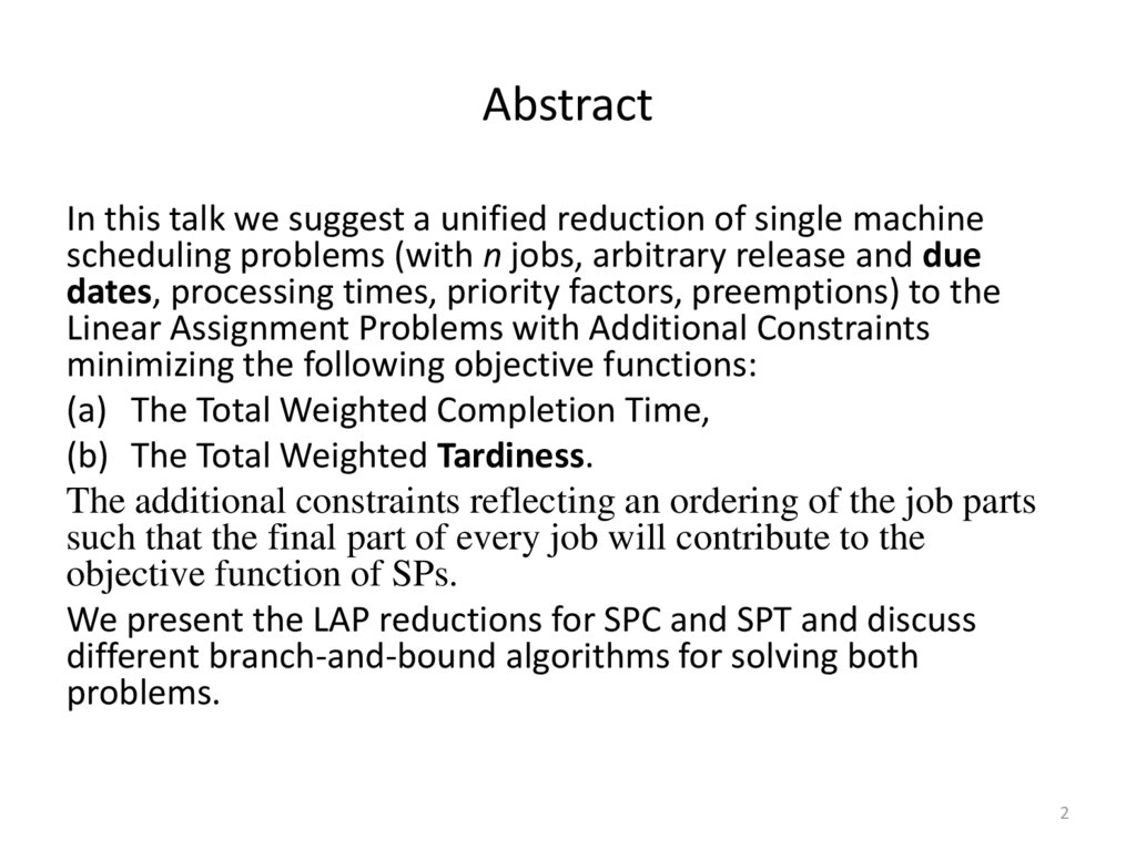
In this talk we suggest a unified reduction of single machinescheduling problems (with n jobs, arbitrary release and due
dates, processing times, priority factors, preemptions) to the
Linear Assignment Problems with Additional Constraints
minimizing the following objective functions:
(a) The Total Weighted Completion Time,
(b) The Total Weighted Tardiness.
The additional constraints reflecting an ordering of the job parts
such that the final part of every job will contribute to the
objective function of SPs.
We present the LAP reductions for SPC and SPT and discuss
different branch-and-bound algorithms for solving both
problems.
2
3. Our Results
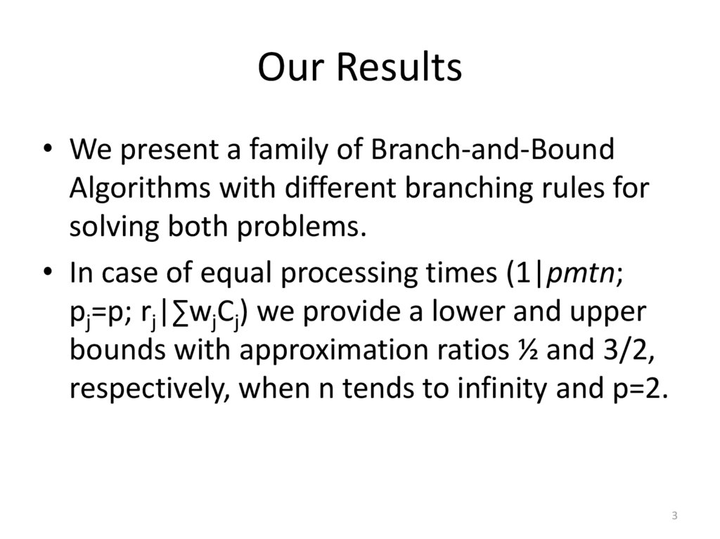
• We present a family of Branch-and-BoundAlgorithms with different branching rules for
solving both problems.
• In case of equal processing times (1|pmtn;
pj=p; rj|∑wjCj) we provide a lower and upper
bounds with approximation ratios ½ and 3/2,
respectively, when n tends to infinity and p=2.
3
4. Two Single Machine Scheduling Problems
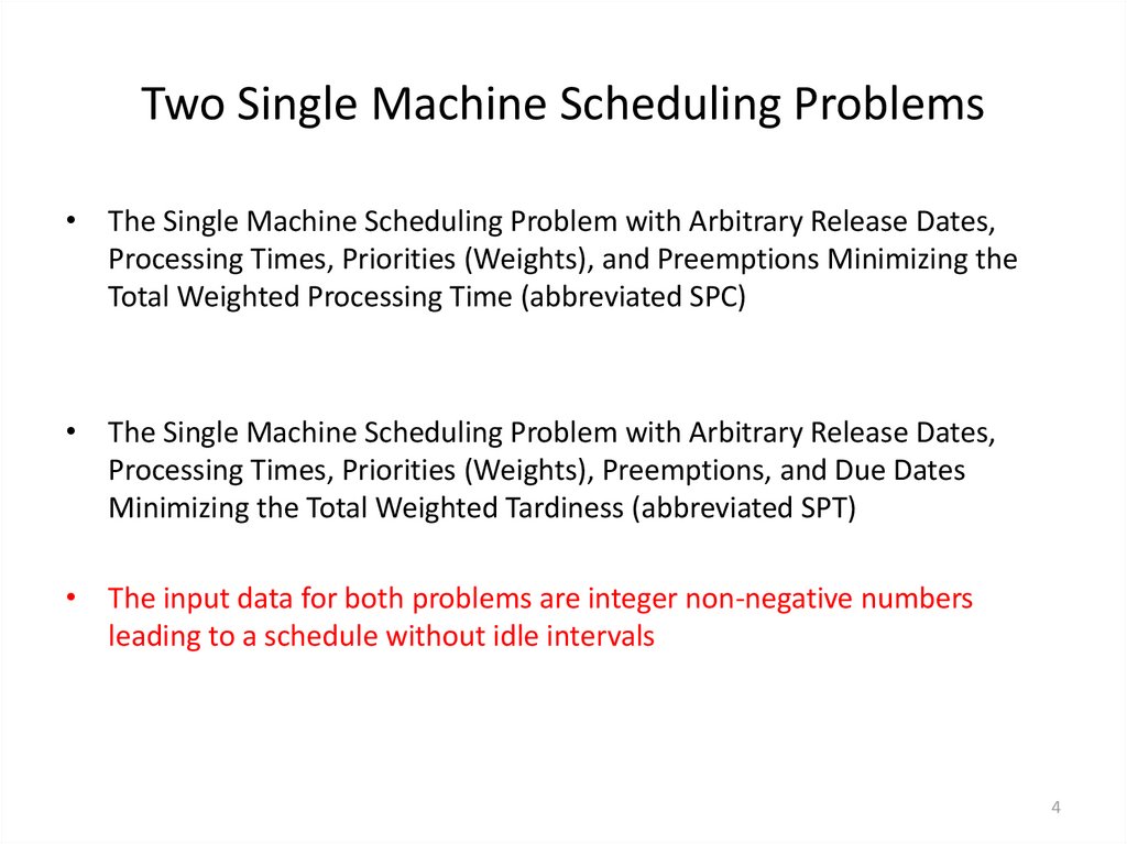
• The Single Machine Scheduling Problem with Arbitrary Release Dates,Processing Times, Priorities (Weights), and Preemptions Minimizing the
Total Weighted Processing Time (abbreviated SPC)
• The Single Machine Scheduling Problem with Arbitrary Release Dates,
Processing Times, Priorities (Weights), Preemptions, and Due Dates
Minimizing the Total Weighted Tardiness (abbreviated SPT)
• The input data for both problems are integer non-negative numbers
leading to a schedule without idle intervals
4
5. An example: schedule 3 jobs to minimize either the total weighted completion time or total weighted tardiness.
jpj
1
2
2
3
3
2
wj
2
8
10
rj
1
2
dj
1
3
3
3
Since both problems are NP-hard (computationally intractable)
we are going to design heuristics and exact algorithms.
5
6. Informal Reduction to the LAP
A feasible solution of the scheduling problem SPC can berepresented as an assignment of np job parts (each of n jobs has p
parts) to np time intervals 1, 2,...,np such that every part of job j is
assigned to a time interval not earlier than its release date rj . Only
the last (p-th) part of every job j is taken into account in the objective
function. The cost of its assignment to time t is equal wj t, and the
costs for parts 1, 2,...,p − 1 are all equal to 0. The objective is to minimize the total cost over all jobs. Thus, SPC problem is equivalent to
the linear assignment problem with additional constraints related to
release dates rj and also to the sequence of job parts which requires
the last part of a job to be assigned to the latest time interval
among the time intervals of all its parts. Moreover, release date
constraints can be taken into account in the linear assignment
problem using in nite costs for the time intervals to which job parts
cannot be assigned. For the example at next page, the assignment
problem will have the cost matrix shown at the next page.
6
7. Example 1|pmtn; pj=p; rj|∑wjCj
n = 3, p = 4, wj = 1, 2, 3, rj = 1, 4, 7.j
1
2
3
pj
4
4
4
wj
1
2
3
rj
1
4
dj
1
3
7
3
7
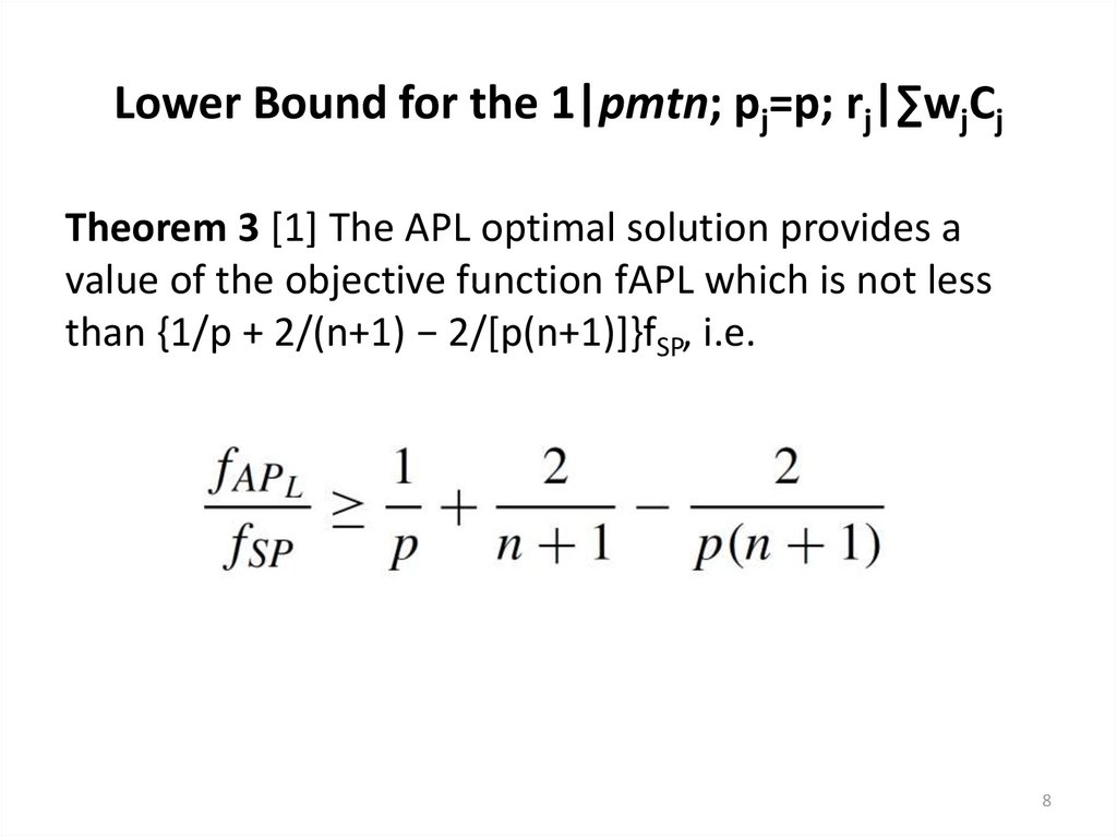
8. Lower Bound for the 1|pmtn; pj=p; rj|∑wjCj
Theorem 3 [1] The APL optimal solution provides avalue of the objective function fAPL which is not less
than {1/p + 2/(n+1) − 2/[p(n+1)]}fSP, i.e.
8
9. LAP Based Upper Bound
• The main drawback of the LAP that it does notinclude the sequence constraints. To
incorporate the sequence constraints, we set
the assignment costs cit to be equal to
w[(i−1)/p]+1t not only for the last part of a job
(when i mod p = 0) but for all its parts. The
corresponding matrix for our example is
shown at then next slide.
9
10. Another Reduction of SPC to the LAP
The optimal assignment problem solution is highlighted withgray color. Now it satis es all the constraints of the original SPC
problem. Unfortunately, it is not an optimal solution to the SPC
problem, because its objective function (OF) is different from
OF of the SPC.
10
11. LAP based Upper Bound [1]
Theorem 611
12. Branch and Bound (BnB) Algorithms for the SPT
• In the next slides we are going to present BnB algorithmsfor solving the SPT exactly by means of different
Branching Rules (BRs).
• There are many BRs:
(i) branch by an infeasible final part of a job with the largest
contribution to the objective function (OF),
(ii) branch by an infeasible not final part of a job with the largest
potential contribution to the OF,
(iii) Branch by tolerance based branching rule.
12
13. Heuristics in BnB Algorithms
• We are going to incorporate an efficient heuristic forthe SPC based on the Weighted Shortest Remaining
Processing Time (WSRPT) rule.
• The computational complexity of our heuristic is
based on the WSRPT rule which is O(n) on each step
of the heuristic. Since there are no idle time intervals
the total number of steps is not greater than npmax.
The WSRPT heuristic stores in memory at most nwj/ρj
ratios. So the heuristic has time complexity of
O(n^2pmax) and space complexity of O(n).
13
14. WSRPT rule: Computational Study
The computational experiments are performed on Inteli7 machine with 2.50 GHz and 8 GB of memory. Our
heuristic is fast enough to solve problems with the
number of jobs n = 1000 and the processing times up pj
∼ 1000 in 10 s. For the greater number of jobs n =
10,000 and pj ∼ 10,000 the algorithm needs about 3 h.
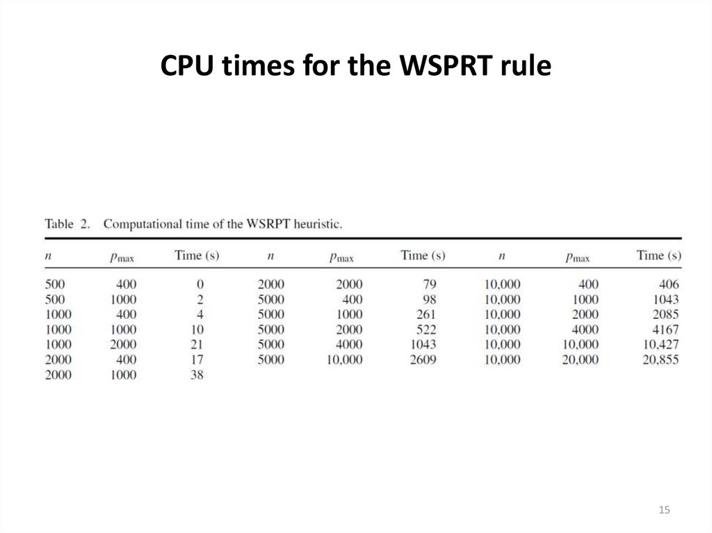
Average computation times for randomly generated
instances are given in Table 2. The average time is
computed on 50 instances.
14
15. CPU times for the WSPRT rule
1516. Quality of the WSRPT rule
To test the quality of heuristic solutions we take n from set {5, 10, 15,20, 25} and pj ∈[1, 100]. For each n we randomly generated 50
instances in the way described above. Every instance is solved exactly
by CPLEX 12 using the BLP model and by the WSRPT heuristic. Then we
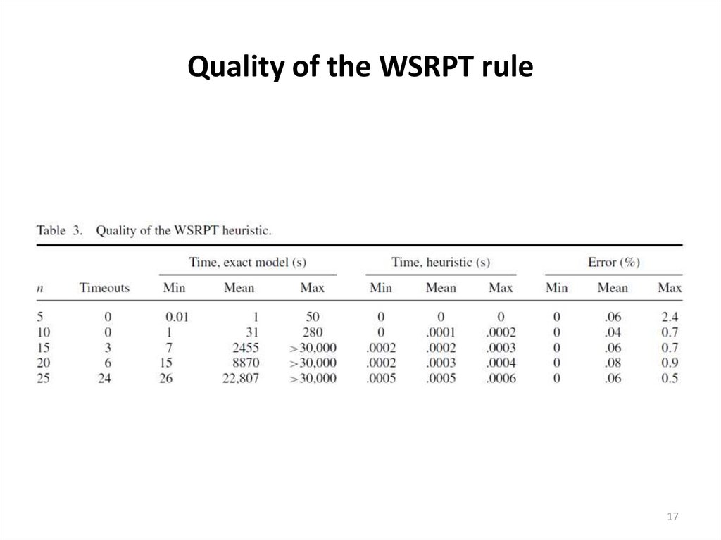
compute the minimum, average, and maximum relative error of the
heuristic solutions over the 50 instances. The results are presented in
Table 3. As it can be seen the WSRPT heuristic nds solutions of high
quality and the average error does not exceed 0.08% for any
combination of n and pj values. We have not considered large values
for n because even for n = 25 half of the instances have not been
solved in 30,000 s (about 8 h) by the CPLEX. The 50 generated
instances for n = 25 have required more than 360 h (15 days) to be
solved exactly. We present the results only for pj ∈[1, 100] because for
smaller values of pj the average and maximal error are virtually the
same and for greater values the errors are even smaller.
16
17. Quality of the WSRPT rule
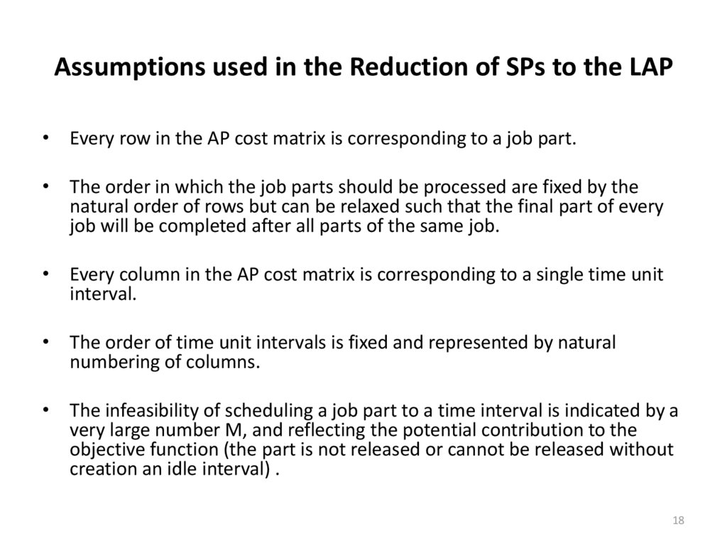
1718. Assumptions used in the Reduction of SPs to the LAP
• Every row in the AP cost matrix is corresponding to a job part.• The order in which the job parts should be processed are fixed by the
natural order of rows but can be relaxed such that the final part of every
job will be completed after all parts of the same job.
• Every column in the AP cost matrix is corresponding to a single time unit
interval.
• The order of time unit intervals is fixed and represented by natural
numbering of columns.
• The infeasibility of scheduling a job part to a time interval is indicated by a
very large number M, and reflecting the potential contribution to the
objective function (the part is not released or cannot be released without
creation an idle interval) .
18
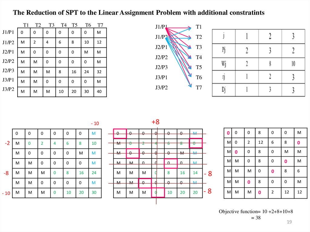
19. The Reduction of SPT to the Linear Assignment Problem with additional constratints
T1T2
T3
T4 T5
T6
T7
J1/P1
0
0
0
0
0
0
M
J1/P2
M
2
4
6
8
10
12
J2/P1
M
0
0
0
0
M
M
J2/P2
M
M
0
0
0
0
M
J2/P3
M
M
M
8
16
24
32
J3/P1
M
M
0
0
0
0
M
J3/P2
M
M
M
10
20
30
40
-8
- 10
T1
J1/P2
T2
J2/P1
T3
J2/P2
T4
J2/P3
T5
J3/P1
T6
J3/P2
T7
+8
- 10
-2
J1/P1
0
0
0
0
0
0
M
0
0
0
0
0
0
M
0 0
0
8
0
0
M
M
0
2
4
6
8
10
M
0
2
4
6
8
0
M 0
2
12
6
8
0
M
0
0
0
0
M
M
M
0
0
0
0
M
M
M 0
0
8
0
M
M
M
M
0
0
0
0
M
M
M
0
0
0
0
M
M M
0
8
0
0
M
M
M
M
0
8
16
24
M
M
M
0
8
16
14
M M
M
0
0
8
6
M
M
0
0
0
0
M
M
M
0
0
0
0
M
M M
0
8
0
0
M
M
M
M
0
10
20
30
M
M
M
0
10
20
20
M M
M
0
2
12
12
-8
-8
Objective function= 10 +2+8+10+8
= 38
19
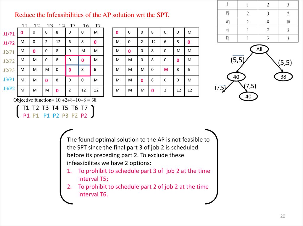
20. Reduce the Infeasibilities of the AP solution wrt the SPT.
J1/P1T1 T2
0
0
T3
T4 T5
T6
T7
0
8
0
0
M
0
0
0
8
0
0
M
J1/P2
M
0
2
12
6
8
0
M
0
2
12
6
8
0
J2/P1
M
0
0
8
0
M
M
M
0
0
8
0
M
M
J2/P2
M
M
0
8
0
0
M
M
M
0
8
0
0
M
J2/P3
M
M
M
0
0
8
6
M
M
M
0
M
8
6
J3/P1
M
M
0
8
0
0
M
M
M
0
8
0
0
M
J3/P2
M
M
M
0
2
12
12
M
M
M
0
2
12
12
Objective function= 10 +2+8+10+8 = 38
All
(7,5)
(5,5)
(5,5)
40
38
(7,5)
40
T1 T2 T3 T4 T5 T6 T7
P1 P1 P1 P2 P3 P2 P2
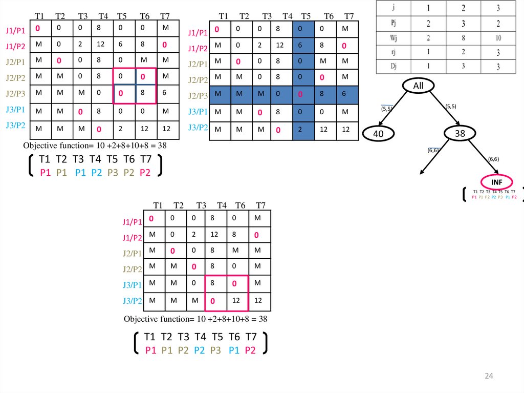
The found optimal solution to the AP is not feasible to
the SPT since the final part 3 of job 2 is scheduled
before its preceding part 2. To exclude these
infeasibilites we have 2 options:
1. To prohibit to schedule part 3 of job 2 at the time
interval T5;
2. To prohibit to schedule part 2 of job 2 at the time
interval T6.
20
21. Reduce the Infeasibilities of the AP solution wrt the SPT.
J1/P1T1 T2
0
0
T3
T4 T5
T6
T7
0
8
0
0
M
0
0
0
8
0
0
M
J1/P2
M
0
2
12
6
8
0
M
0
2
12
6
8
0
J2/P1
M
0
0
8
0
M
M
M
0
0
8
0
M
M
J2/P2
M
M
0
8
0
0
M
M
M
0
8
0
0
M
J2/P3
M
M
M
0
0
8
6
M
M
M
0
M
8
6
J3/P1
M
M
0
8
0
0
M
M
M
0
8
0
0
M
J3/P2
M
M
M
0
2
12
12
M
M
M
0
2
12
12
All
(7,5)
(5,5)
(5,5)
40
38
(7,5)
40
Objective function= 10 +2+8+10+8 = 38
T1 T2 T3 T4 T5 T6 T7
P1 P1 P1 P2 P3 P2 P2
T1 T2
0
J1/P1 0
T3
T4 T5
T6
T7
0
8
0
0
M
J1/P2 M
0
2
12
6
8
0
J2/P1 M
0
0
8
0
M
M
J2/P2 M
M
0
8
0
0
M
J2/P3 M
M
M
0
M
6
4
J3/P1 M
M
0
2
0
0
M
J3/P2 M
M
M
0
0
10
10
Objective function= 38+2 = 40
T1 T2 T3 T4 T5 T6 T7
P1 P1 P2 P3 P2 P1 P2
21
22.
T1T2
T3
T4 T5
T6
T7
0
0
0
12
0
0
M
M
0
2
16
6
8
0
J2/P1 M
0
0
12
0
M
M
J2/P2 M
M
0
12
0
0
M
J2/P3 M
M
M
0
M
2
0
J3/P1 M
M
0
6
0
0
M
J3/P2 M
M
M
0
M
6
6
J1/P1
J1/P2
Objective function= 40+4= 44
T1 T2 T3 T4 T5 T6 T7
P1 P2 P1 P2 P1 P2 P3
T1
T2
T3
T4 T5
T6
T7
J1/P1
0
0
0
8
0
0
M
J1/P2
M
0
2
12
6
8
0
J2/P1
M
0
0
8
0
M
M
J2/P2
M
M
0
8
0
0
M
J2/P3
M
M
M
0
M
6
4
J3/P1
M
M
0
2
0
0
M
J3/P2
M
M
M
0
0
10
10
All
(7,5)
44
(5,5)
(5,5)
40
38
(7,5)
40
T1 T2 T3 T4 T5 T6 T7
P1 P2 P1 P2 P1 P2 P3
Objective function= 38+2 = 40
T1 T2 T3 T4 T5 T6 T7
P1 P1 P2 P3 P2 P1 P2
22
23.
T1T2
T3
T4 T5
T6
T7
J1/P1
0
0
0
8
0
0
M
J1/P2
M
0
2
12
6
8
0
J2/P1
M
0
0
8
0
M
M
J2/P2
M
M
0
8
0
0
M
J2/P3
M
M
M
0
M
6
4
J3/P1
M
M
0
2
0
0
M
J3/P2
M
M
M
0
M
10
10
All
(5,5)
(5,5)
38
40
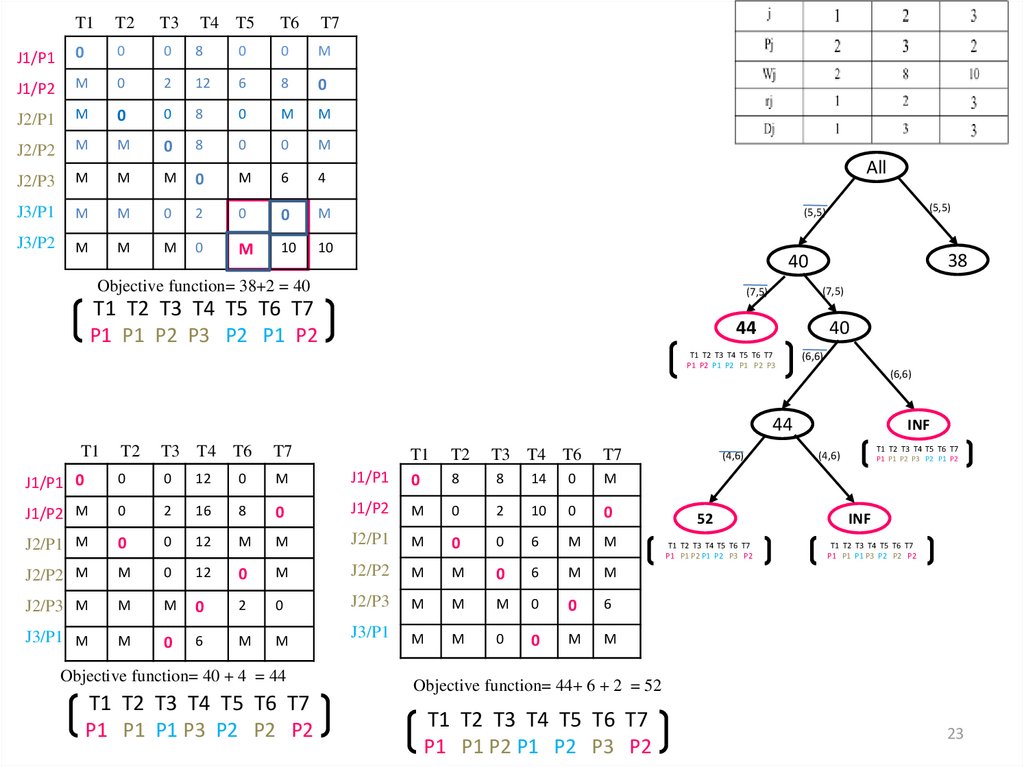
Objective function= 38+2 = 40
(7,5)
(7,5)
T1 T2 T3 T4 T5 T6 T7
P1 P1 P2 P3 P2 P1 P2
40
44
T1 T2 T3 T4 T5 T6 T7
P1 P2 P1 P2 P1 P2 P3
(6,6)
(6,6)
44
T1
T2
T3 T4 T6
T7
J1/P1 0
0
0
12
0
M
J1/P2 M
0
2
16
8
T2
J1/P1
T1
0
T3 T4 T6
T7
8
8
14
0
M
0
J1/P2
M
0
2
10
0
0
M
0
0
6
M
M
J2/P1 M
0
0
12
M
M
J2/P1
J2/P2 M
M
0
12
0
M
J2/P2
M
M
0
6
M
M
J2/P3 M
M
M
0
2
0
J2/P3
M
M
M
0
0
6
J3/P1 M
M
0
6
M
M
J3/P1
M
M
0
0
M
M
Objective function= 40 + 4 = 44
T1 T2 T3 T4 T5 T6 T7
P1 P1 P1 P3 P2 P2 P2
(4,6)
52
T1 T2 T3 T4 T5 T6 T7
P1 P1 P2 P1 P2 P3 P2
INF
T1 T2 T3 T4 T5 T6 T7
(4,6)
P1 P1 P2 P3 P2 P1 P2
INF
T1 T2 T3 T4 T5 T6 T7
P1 P1 P1 P3 P2 P2 P2
Objective function= 44+ 6 + 2 = 52
T1 T2 T3 T4 T5 T6 T7
P1 P1 P2 P1 P2 P3 P2
23
24.
T2T3
T4 T5
T6
T7
J1/P1
T1
0
M
T1 T2 T3 T4 T5
0
0
8
0
J1/P1 0
0
0
8
0
0
J1/P2
M
0
2
12
6
J2/P1
M
0
0
8
J2/P2
M
M
0
J2/P3
M
M
J3/P1
M
J3/P2
M
0
M
8
0
J1/P2 M
0
2
12
6
8
0
0
M
M
J2/P1 M
0
0
8
0
M
M
8
0
0
M
J2/P2 M
M
0
8
0
0
M
M
0
0
8
6
J2/P3 M
M
M
0
0
8
6
M
0
8
0
0
M
J3/P1 M
M
0
8
0
0
M
M
M
0
2
12
12
J3/P2 M
M
M
0
2
12
12
Objective function= 10 +2+8+10+8 = 38
T6
T7
All
(5,5)
(5,5)
38
40
(6,6)
T1 T2 T3 T4 T5 T6 T7
(6,6)
P1 P1 P1 P2 P3 P2 P2
INF
T1 T2 T3 T4 T5 T6 T7
P1 P1 P2 P2 P3 P1 P2
T1 T2 T3 T4 T6
0
0
8
0
J1/P1 0
T7
M
J1/P2 M
0
2
12
8
0
J2/P1 M
0
0
8
M
M
J2/P2 M
M
0
8
0
M
J3/P1 M
M
0
8
0
M
J3/P2 M
M
M
0
12
12
Objective function= 10 +2+8+10+8 = 38
T1 T2 T3 T4 T5 T6 T7
P1 P1 P2 P2 P3 P1 P2
24
25.
T1 T2 T3 T4 T60
0
8
0
0
M
J1/P2
M
0
2
4
0
0
J2/P1
M
0
0
0
M
M
J2/P2
M
M
0
8
0
M
J3/P1
M
M
0
0
M
M
J3/P2
M
M
M
0
12
12
J1/P1
T7
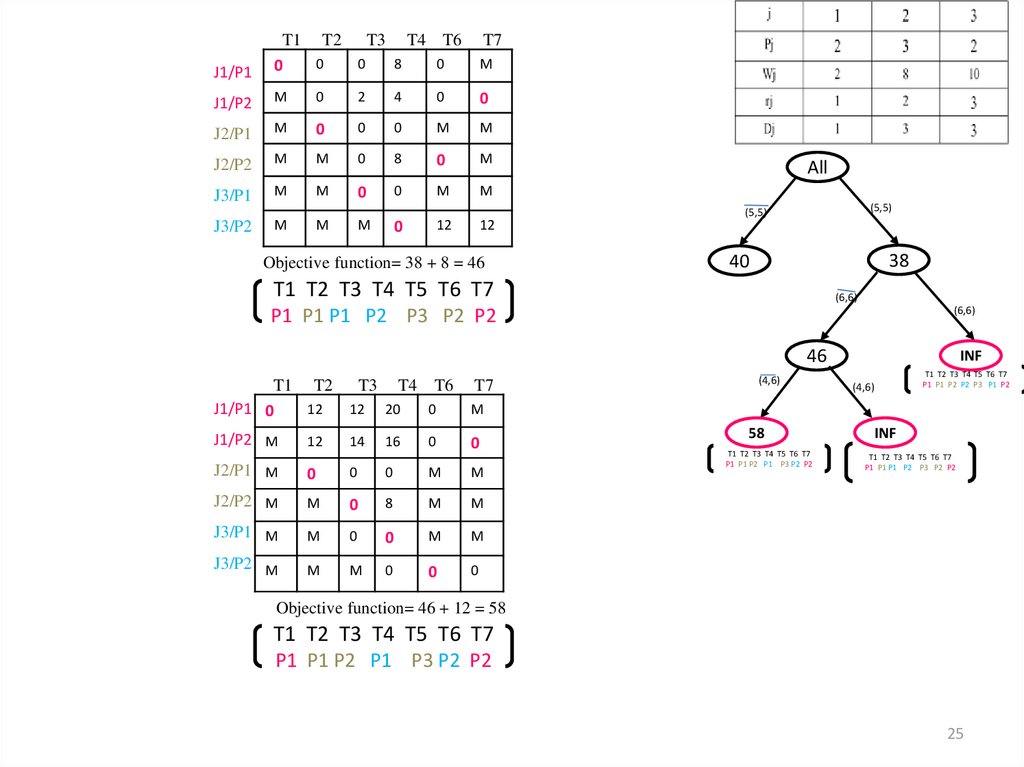
Objective function= 38 + 8 = 46
All
(5,5)
(5,5)
38
40
T1 T2 T3 T4 T5 T6 T7
(6,6)
(6,6)
P1 P1 P1 P2 P3 P2 P2
46
T1 T2 T3 T4 T6
12
12 20
0
J1/P1 0
M
J1/P2 M
0
12
14
16
0
T7
J2/P1 M
0
0
0
M
M
J2/P2 M
M
0
8
M
M
J3/P1 M
M
0
0
M
M
J3/P2 M
M
M
0
0
0
(4,6)
58
T1 T2 T3 T4 T5 T6 T7
P1 P1 P2 P1 P3 P2 P2
INF
(4,6)
T1 T2 T3 T4 T5 T6 T7
P1 P1 P2 P2 P3 P1 P2
INF
T1 T2 T3 T4 T5 T6 T7
P1 P1 P1 P2 P3 P2 P2
Objective function= 46 + 12 = 58
T1 T2 T3 T4 T5 T6 T7
P1 P1 P2 P1 P3 P2 P2
25
26.
T1 T20
0
0
8
0
0
M
J1/P2
M
0
2
12
6
8
0
J2/P1
M
0
0
8
0
M
M
J2/P2
M
M
0
8
0
0
M
J2/P3
M
M
M
0
0
8
6
J3/P1
M
M
0
8
0
0
M
J3/P2
M
M
M
0
2
12
12
J1/P1
T3
T4 T5
T6
T7
All
(5,5)
(5,5)
38
40
(7,5)
(7,5)
(6,6)
40
44
T1 T2 T3 T4 T5 T6 T7
P1 P2 P1 P2 P1 P2 P3
46
(6,6)
(6,6)
44
(4,6)
52
T1 T2 T3 T4 T5 T6 T7
P1 P1 P2 P1 P2 P3 P2
INF
(4,6)
(6,6)
T1 T2 T3 T4 T5 T6 T7
P1 P1 P2 P3 P2 P1 P2
(4,6)
58
T1 T2 T3 T4 T5 T6 T7
P1 P1 P2 P1 P3 P2 P2
INF
(4,6)
T1 T2 T3 T4 T5 T6 T7
P1 P1 P2 P2 P3 P1 P2
INF
T1 T2 T3 T4 T5 T6 T7
P1 P1 P1 P2 P3 P2 P2
INF
T1 T2 T3 T4 T5 T6 T7
P1 P1 P1 P3 P2 P2 P2
26
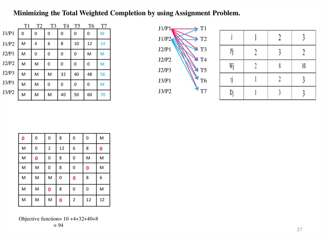
27. Minimizing the Total Weighted Completion by using Assignment Problem.
T1T2
T3
T4 T5
T6
T7
J1/P1
0
0
0
0
0
0
M
J1/P2
M
4
6
8
10
12
14
J2/P1
M
0
0
0
0
M
M
J2/P2
M
M
0
0
0
0
M
J2/P3
M
M
M
32
40
48
56
J3/P1
M
M
0
0
0
0
M
J3/P2
M
M
M
40
50
60
70
0
0
0
8
0
0
M
M
0
2
12
6
8
0
M
0
0
8
0
M
M
M
M
0
8
0
0
M
M
M
M
0
0
8
6
M
M
0
8
0
0
M
M
M
M
0
2
12
12
Objective function= 10 +4+32+40+8
= 94
J1/P1
T1
J1/P2
T2
J2/P1
T3
J2/P2
T4
J2/P3
T5
J3/P1
T6
J3/P2
T7
27
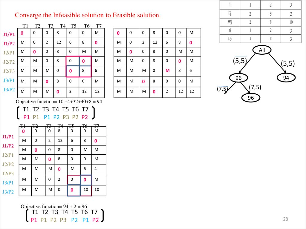
28. Converge the Infeasible solution to Feasible solution.
J1/P1T1 T2
0
0
T3
T4 T5
T6
T7
0
8
0
0
M
0
0
0
8
0
0
M
J1/P2
M
0
2
12
6
8
0
M
0
2
12
6
8
0
J2/P1
M
0
0
8
0
M
M
M
0
0
8
0
M
M
J2/P2
M
M
0
8
0
0
M
M
M
0
8
0
0
M
J2/P3
M
M
M
0
0
8
6
M
M
M
0
M
8
6
J3/P1
M
M
0
8
0
0
M
M
M
0
8
0
0
M
J3/P2
M
M
M
0
2
12
12
M
M
M
0
2
12
12
Objective function= 10 +4+32+40+8 = 94
All
(7,5)
(5,5)
(5,5)
96
94
(7,5)
96
T1 T2 T3 T4 T5 T6 T7
P1 P1 P1 P2 P3 P2 P2
J1/P1
J1/P2
J2/P1
J2/P2
T1
0
T2
T3
T6
T7
0
0
8
0
0
M
M
0
2
12
6
8
0
M
0
0
8
0
M
M
M
M
0
8
0
0
M
M
M
M
0
M
6
4
M
M
0
2
0
0
M
M
M
M
0
0
10
10
J2/P3
J3/P1
J3/P2
T4 T5
Objective function= 94 + 2 = 96
T1 T2 T3 T4 T5 T6 T7
P1 P1 P2 P3 P2 P1 P2
28
29.
T4 T5T6
T7
0
12
0
0
M
0
2
16
6
8
0
J2/P1 M
0
0
12
0
M
M
J2/P2 M
M
0
12
0
0
M
J2/P3 M
M
M
0
M
2
0
J3/P1 M
M
0
6
0
0
M
J3/P2 M
M
M
0
M
6
6
J1/P1
J1/P2
T1
T2
T3
0
0
M
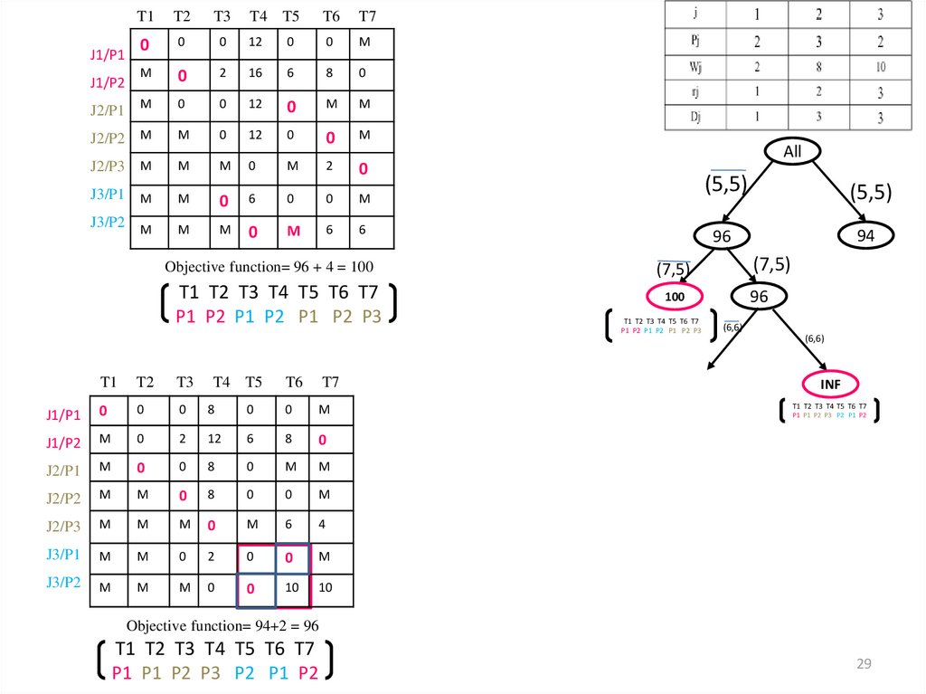
Objective function= 96 + 4 = 100
T1 T2 T3 T4 T5 T6 T7
P1 P2 P1 P2 P1 P2 P3
T1
T2
T3
T4 T5
T6
T7
J1/P1
0
0
0
8
0
0
M
J1/P2
M
0
2
12
6
8
0
J2/P1
M
0
0
8
0
M
M
J2/P2
M
M
0
8
0
0
M
J2/P3
M
M
M
0
M
6
4
J3/P1
M
M
0
2
0
0
M
J3/P2
M
M
M
0
0
10
10
All
(5,5)
(5,5)
96
94
(7,5)
(7,5)
96
100
T1 T2 T3 T4 T5 T6 T7
P1 P2 P1 P2 P1 P2 P3
(6,6)
(6,6)
INF
T1 T2 T3 T4 T5 T6 T7
P1 P1 P2 P3 P2 P1 P2
Objective function= 94+2 = 96
T1 T2 T3 T4 T5 T6 T7
P1 P1 P2 P3 P2 P1 P2
29
30.
T1T2
T3
T4 T5
T6
T7
J1/P1
0
0
0
8
0
0
M
J1/P2
M
0
2
12
6
8
0
J2/P1
M
0
0
8
0
M
M
J2/P2
M
M
0
8
0
0
M
J2/P3
M
M
M
0
M
6
4
J3/P1
M
M
0
2
0
0
M
J3/P2
M
M
M
0
0
10
10
All
(5,5)
(5,5)
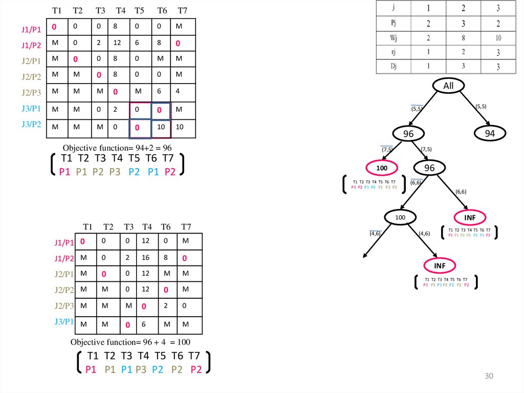
Objective function= 94+2 = 96
(7,5)
(7,5)
T1 T2 T3 T4 T5 T6 T7
P1 P1 P2 P3 P2 P1 P2
94
96
96
100
T1 T2 T3 T4 T5 T6 T7
P1 P2 P1 P2 P1 P2 P3
(6,6)
(6,6)
INF
100
T1
T2
T3 T4 T6
T7
J1/P1 0
0
0
12
0
M
J1/P2 M
0
2
16
8
0
J2/P1 M
0
0
12
M
M
J2/P2 M
M
0
12
0
M
J2/P3 M
M
M
0
2
0
J3/P1 M
M
0
6
M
M
(4,6)
T1 T2 T3 T4 T5 T6 T7
(4,6)
P1 P1 P2 P3 P2 P1 P2
INF
T1 T2 T3 T4 T5 T6 T7
P1 P1 P1 P3 P2 P2 P2
Objective function= 96 + 4 = 100
T1 T2 T3 T4 T5 T6 T7
P1 P1 P1 P3 P2 P2 P2
30
31.
T2J1/P1
T1
0
T3 T4 T6
T7
8
8
14
0
M
J1/P2
M
0
2
10
0
0
J2/P1
M
0
0
6
M
M
J2/P2
M
M
0
6
M
M
J2/P3
M
M
M
0
0
6
J3/P1
M
M
0
0
M
M
All
(5,5)
(5,5)
(7,5)
(7,5)
96
100
Objective function= 100+ 6 + 2 =108
T1 T2 T3 T4 T5 T6 T7
P1 P1 P2 P1 P2 P3 P2
94
96
T1 T2 T3 T4 T5 T6 T7
P1 P2 P1 P2 P1 P2 P3
(6,6)
(6,6)
INF
100
(4,6)
108
T1 T2 T3 T4 T5 T6 T7
P1 P1 P2 P1 P2 P3 P2
T1 T2 T3 T4 T5 T6 T7
(4,6)
P1 P1 P2 P3 P2 P1 P2
INF
T1 T2 T3 T4 T5 T6 T7
P1 P1 P1 P3 P2 P2 P2
31
32.
T2T3
T4 T5
T6
T7
J1/P1
T1
0
M
T1 T2 T3 T4 T5
0
0
8
0
J1/P1 0
0
0
8
0
0
J1/P2
M
0
2
12
6
J2/P1
M
0
0
8
J2/P2
M
M
0
J2/P3
M
M
J3/P1
M
J3/P2
M
0
M
8
0
J1/P2 M
0
2
12
6
8
0
0
M
M
J2/P1 M
0
0
8
0
M
M
8
0
0
M
J2/P2 M
M
0
8
0
0
M
M
0
0
8
6
J2/P3 M
M
M
0
0
8
6
M
0
8
0
0
M
J3/P1 M
M
0
8
0
0
M
M
M
0
2
12
12
J3/P2 M
M
M
0
2
12
12
Objective function= 10 +4+32+40+8 = 94
T1 T2 T3 T4 T5 T6 T7
P1 P1 P1 P2 P3 P2 P2
T6
T7
All
(5,5)
(5,5)
94
96
(6,6)
(6,6)
INF
T1 T2 T3 T4 T5 T6 T7
P1 P1 P2 P2 P3 P1 P2
T1 T2 T3 T4 T6
0
0
8
0
J1/P1 0
T7
M
J1/P2 M
0
2
12
8
0
J2/P1 M
0
0
8
M
M
J2/P2 M
M
0
8
0
M
J3/P1 M
M
0
8
0
M
J3/P2 M
M
M
0
12
12
Objective function= 10 +4+32+40+8 = 94
T1 T2 T3 T4 T5 T6 T7
P1 P1 P2 P2 P3 P1 P2
32
33.
T1 T2 T3 T4 T60
0
8
0
0
M
J1/P2
M
0
2
4
0
0
J2/P1
M
0
0
0
M
M
J2/P2
M
M
0
8
0
M
J3/P1
M
M
0
0
M
M
J3/P2
M
M
M
0
12
12
J1/P1
T7
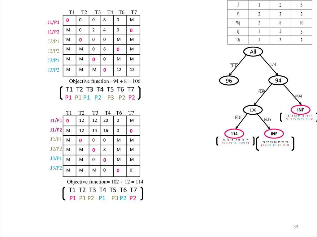
Objective function= 94 + 8 = 106
All
(5,5)
(5,5)
94
96
T1 T2 T3 T4 T5 T6 T7
(6,6)
(6,6)
P1 P1 P1 P2 P3 P2 P2
T1
J1/P1 0
T2
T3
T4 T6
12
12
20
0
M
J1/P2 M
12
14
16
0
0
J2/P1 M
0
0
0
M
M
J2/P2 M
M
0
8
M
M
J3/P1 M
M
0
0
M
M
J3/P2 M
M
M
0
0
0
INF
106
T7
(4,6)
114
T1 T2 T3 T4 T5 T6 T7
P1 P1 P2 P1 P3 P2 P2
(4,6)
T1 T2 T3 T4 T5 T6 T7
P1 P1 P2 P2 P3 P1 P2
INF
T1 T2 T3 T4 T5 T6 T7
P1 P1 P1 P2 P3 P2 P2
Objective function= 102 + 12 = 114
T1 T2 T3 T4 T5 T6 T7
P1 P1 P2 P1 P3 P2 P2
33
34.
T1 T20
0
0
8
0
0
M
J1/P2
M
0
2
12
6
8
0
J2/P1
M
0
0
8
0
M
M
J2/P2
M
M
0
8
0
0
M
J2/P3
M
M
M
0
0
8
6
J3/P1
M
M
0
8
0
0
M
J3/P2
M
M
M
0
2
12
12
J1/P1
T3
T4 T5
T6
T7
All
(5,5)
(5,5)
94
94
(7,5)
(7,5)
(6,6)
94
100
T1 T2 T3 T4 T5 T6 T7
P1 P2 P1 P2 P1 P2 P3
108
T1 T2 T3 T4 T5 T6 T7
P1 P1 P2 P1 P2 P3 P2
INF
106
(6,6)
(6,6)
INF
100
(4,6)
(6,6)
(4,6)
T1 T2 T3 T4 T5 T6 T7
P1 P1 P2 P3 P2 P1 P2
(4,6)
114
T1 T2 T3 T4 T5 T6 T7
P1 P1 P2 P1 P3 P2 P2
(4,6)
T1 T2 T3 T4 T5 T6 T7
P1 P1 P2 P2 P3 P1 P2
INF
T1 T2 T3 T4 T5 T6 T7
P1 P1 P1 P2 P3 P2 P2
INF
T1 T2 T3 T4 T5 T6 T7
P1 P1 P1 P3 P2 P2 P2
34
35. Summary
• In this talk we have presented the reduction of two singlemachine scheduling problems to the linear assignment
problem with additional constraints.
• The idea of branch-and-bound algorithm with two different
branching rules is outlined.
• Our future computational experiments will show which of
eithe two mentioned or tolerance based branching rules
should be used for solving these SPs.
35
36. Future Research Directions
• We will extend our approach to the following objectivefunctions:
• Minimize the maximum lateness (Lj=Cj – dj);
• Minimize the makespan (Cmax);
• Minimize the weighted number of tardy jobs;
• Minimize the total weighted earliness (note that the earliness penalty is
nonincreasing in Cj (Ej=max{dj – Cj, 0}).
• Minimize the linear combination of the total weighted earliness and the
total weighted tardiness with arbitrary weights.
• We will design tolerance based branching rules and bounds
with the purpose to reduce the total CPU times compared to
the costs based counterparts.
36
37. References
• 1. M. Batsyn, B. Goldengorin, P. Sukhov, P. M. Pardalos. Lowerand Upper Bounds for the Preemptive Single Machine
Scheduling Problem with Equal Processing Times. Springer
Proceedings in Mathematics & Statistics, Vol. 59, 11–30, 2013.
• 2. M. Batsyn, B. Goldengorin, P. Sukhov, P. M. Pardalos. Online
heuristic for the preemptive single machine scheduling
problem of minimizing the total weighted completion time.
Optimization Methods and Software, 2014, 29(5):955–963.
37
38. Questions?
3839. Thank you!
3940. Old abstract
• Recently Batsyn et al. (2013, 2014) havesuggested a reduction of the SPC and SPT to the
Assignment Problem (AP) with additional
constraints. The additional constraints reflecting
an ordering of the job parts such that the final part
of every job will contribute to the objective
function of SPs.
• In this talk we present the AP reductions for SPC
and SPT and discuss different branch-and-bound
algorithms for solving both problems.
40
41.
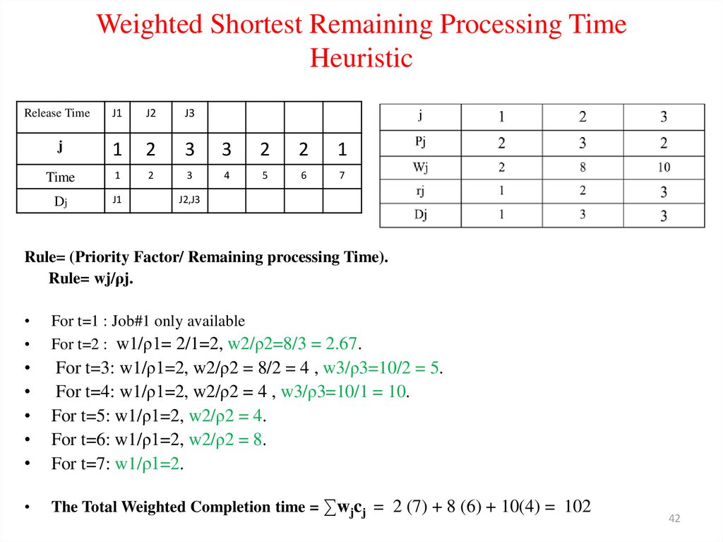
4142. Weighted Shortest Remaining Processing Time Heuristic
J1J2
J3
j
1
2
3
3
2
2
1
Time
1
2
3
4
5
6
7
Dj
J1
Release Time
J2,J3
Rule= (Priority Factor/ Remaining processing Time).
Rule= wj/ρj.
For t=1 : Job#1 only available
For t=2 : w1/ρ1= 2/1=2, w2/ρ2=8/3 = 2.67.
For t=3: w1/ρ1=2, w2/ρ2 = 8/2 = 4 , w3/ρ3=10/2 = 5.
For t=4: w1/ρ1=2, w2/ρ2 = 4 , w3/ρ3=10/1 = 10.
For t=5: w1/ρ1=2, w2/ρ2 = 4.
For t=6: w1/ρ1=2, w2/ρ2 = 8.
For t=7: w1/ρ1=2.
The Total Weighted Completion time = ∑wjcj = 2 (7) + 8 (6) + 10(4) = 102
42




![LAP based Upper Bound [1] LAP based Upper Bound [1]](https://cf2.ppt-online.org/files2/slide/a/A9i6XgfeL71Mbzk2mthSFTQvJuRrxG4DKsIwVC/slide-10.jpg)








 programming


