Business Statistics

1. Business Statistics

2. About Applied Statistics

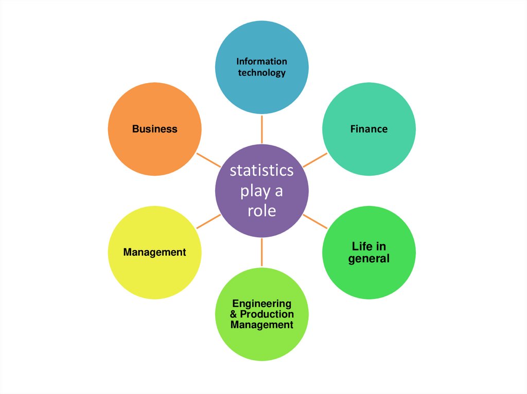
Applied statistics help us decide how best to count and measure, how to
represent numerical information – especially information about groups –
effectively and without misleading ourselves and others, and how to explore
our ideas about relationships among factors that affect quantitative data.
Statistics allow us to summarize large data sets in ways that let us
make sense of what would otherwise be a morass of detail. They let us
test our ideas to see if possible explanations are rooted in reality or
whether they are impression created by the winds of chance
Statistics is often described as the art of decision under uncertainty.

3.

Information
technology
Finance
Business
statistics
play a
role
Life in
general
Management
Engineering
& Production
Management

4. Data Structures Classifying the Various Types of Data Sets

Data can come to you in several different forms, and it
will be useful to have a basic catalog of the different
kinds of data so that you can recognize them and use
appropriate techniques for each. A data set consists of
observations on items, typically with the same
information being recorded for each item.
A piece of information recorded for every item (eg, its
cost) is called a variable. The number of variables
(pieces of information) recorded for each item
indicates the complexity of the data set and will guide
you toward the proper kinds of analyses. Depending
on whether one, two, or many variables are present,
you have univariate, bivariate, or multivariate data,
respectively.

5. Univariate Data

• Univariate (one-variable) data sets have just one piece of
information recorded for each item. Statistical methods are
used to summarize the basic properties of this single piece
of information, answering such questions as:
• 1. What is a typical (summary) value?
• 2. How diverse are these items?
• 3. Do any individuals or groups require special attention?

6. Bivariate Data

Bivariate (two-variable) data sets have exactly two pieces of information
recorded for each item. In addition to summarizing each of these two variables
separately (each as its own univariate data set), statistical methods would also
be used to explore the relationship between the two factors being measured in
the following ways:
1. Is there a simple relationship between the two?
2. How strongly are they related?
3. Can you predict one from the other? If so, with what degree of reliability?
4. Do any individuals or groups require special attention?

7. Multivariate Data

Multivariate Data
Multivariate (many-variable) data sets have three or more pieces of
information recorded for each item. In addition to summarizing each of
these variables separately (as a univariate data set), and in addition to
looking at the relationship between any two variables (as a bivariate data
set), statistical methods would also be used to look at the interrelationships
among all the items, addressing the following questions:
1. Is there a simple relationship among them?
2. How strongly are they related?
3. Can you predict one (a “special variable”) from the others? With what
degree of reliability?
4. Do any individuals or groups require special attention?

8.

Data
QUANTITATIVE
DATA:
NUMBERS
Discrete
Quantitative
Data
Continuous
Quantitative
Data
QUALITATIVE
DATA:
CATEGORIES
Ordinal
Qualitative
Data
Nominal
Qualitative
Data

9. QUANTITATIVE DATA: NUMBERS

• Meaningful numbers are numbers that directly represent the
measured or observed amount of some characteristic or
quality of the elementary units, as the result of an observation
of a variable. Meaningful numbers include, for example, dollar
amounts, counts, sizes, numbers of employees.
• If the data for a variable comes to you as meaningful numbers,
then you have quantitative data (ie, they represent quantities).
With quantitative data, you can do all of the usual numbercrunching tasks, such as finding the average and measuring
the variability.
• It is straightforward to compute directly with numerical data.
• There are two kinds of quantitative data, discrete and
continuous, depending on the values potentially observable.

10.

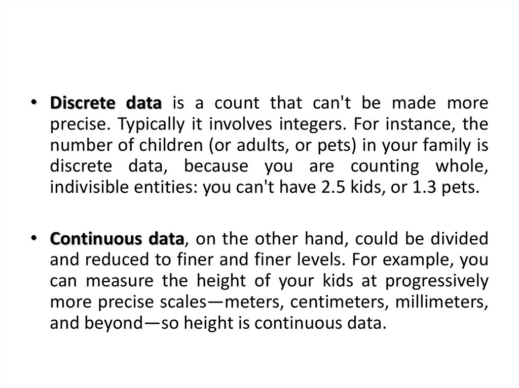
• Discrete data is a count that can't be made more
precise. Typically it involves integers. For instance, the
number of children (or adults, or pets) in your family is
discrete data, because you are counting whole,
indivisible entities: you can't have 2.5 kids, or 1.3 pets.
• Continuous data, on the other hand, could be divided
and reduced to finer and finer levels. For example, you
can measure the height of your kids at progressively
more precise scales—meters, centimeters, millimeters,
and beyond—so height is continuous data.

11. QUALITATIVE DATA: CATEGORIES

• Qualitative data is defined as the data that approximates
and characterizes.
• This data type is non-numerical in nature. This type of
data is collected through methods of observations, oneto-one interview, conducting focus groups and similar
methods.
• Qualitative data in statistics is also known as categorical
data.
• There are two kinds of qualitative data: ordinal (for which
there is a meaningful ordering but no meaningful
numerical assignment) and nominal (for which there is no
meaningful order).

12. Charts, Histograms, Graphing

13.

14. USING A HISTOGRAM TO DISPLAY THE FREQUENCIES

• The histogram displays the frequencies as a bar
chart rising above the number line, indicating how
often the various values occur in the data set. The
horizontal axis represents the measurements of the
data set (eg, in dollars, number of people, miles per
gallon, etc.), and the vertical axis represents how
often these values occur. An especially high bar
indicates that many data values were found at this
position on the horizontal number line, while a
shorter bar indicates a less common value.
• A histogram is a bar chart of the frequencies, not of the
data.

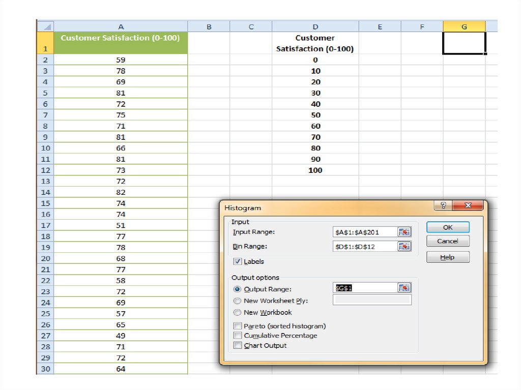
15. Creating Frequency Distributions and Histograms in EXCEL

16.

• Consider the interest rate for 25-year fixed-rate home
mortgages charged by mortgage companies in Seattle

17.

18.

19.

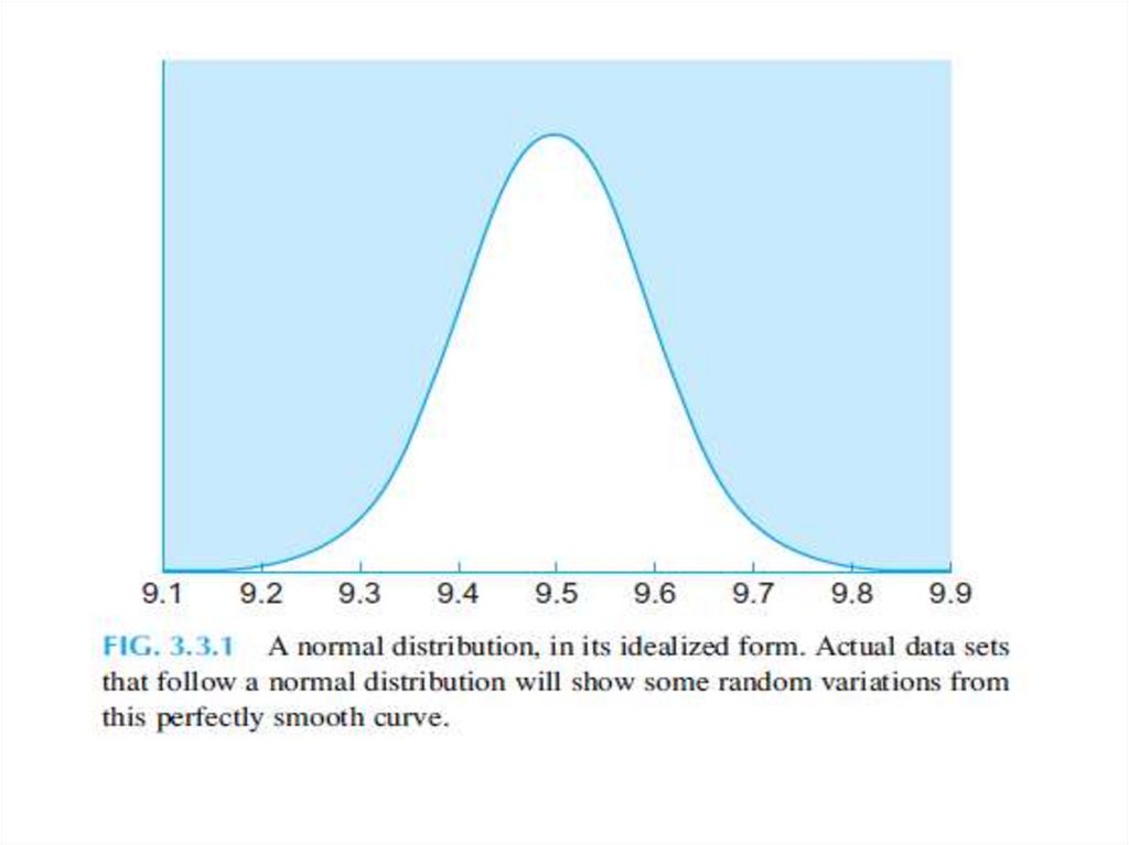
20. NORMAL DISTRIBUTIONS

• A normal distribution is an idealized, smooth,
bell-shaped histogram with all of the
randomness removed. It represents an ideal data
set that has lots of numbers concentrated in the
middle of the range, with the remaining
numbers trailing off symmetrically on both sides.
This degree of smoothness is not attainable by
real data.

21.

22.

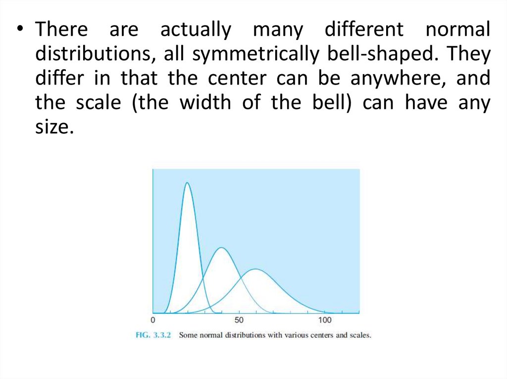
• There are actually many different normal
distributions, all symmetrically bell-shaped. They
differ in that the center can be anywhere, and
the scale (the width of the bell) can have any
size.

23.

24. BIMODAL DISTRIBUTIONS WITH TWO GROUPS

• It is important to be able to recognize when a data set consists
of two or more distinct groups so that they may be analyzed
separately, if appropriate. This can be seen in a histogram as a
distinct gap between two cohesive groups of bars. When two
clearly separate groups are visible in a histogram, you have a
bimodal distribution. Literally, a bimodal distribution has two
modes, or two distinct clusters of data.

25.

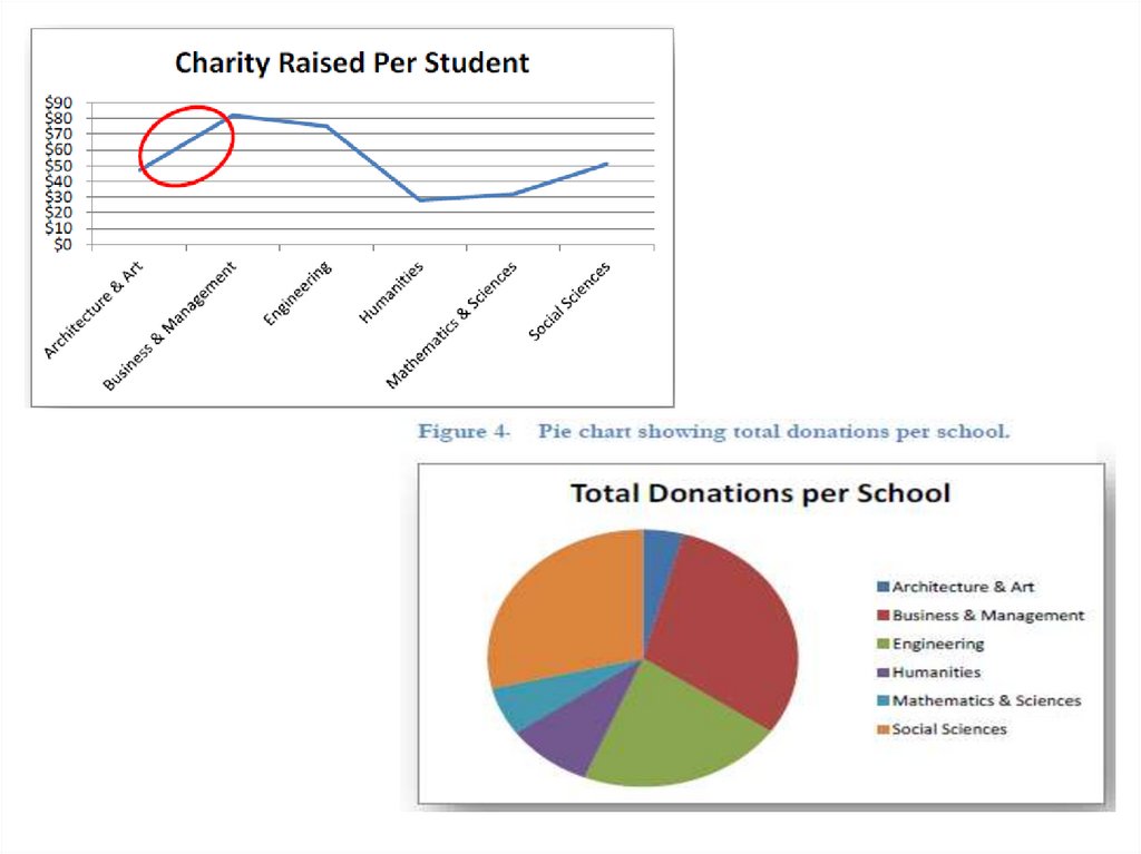
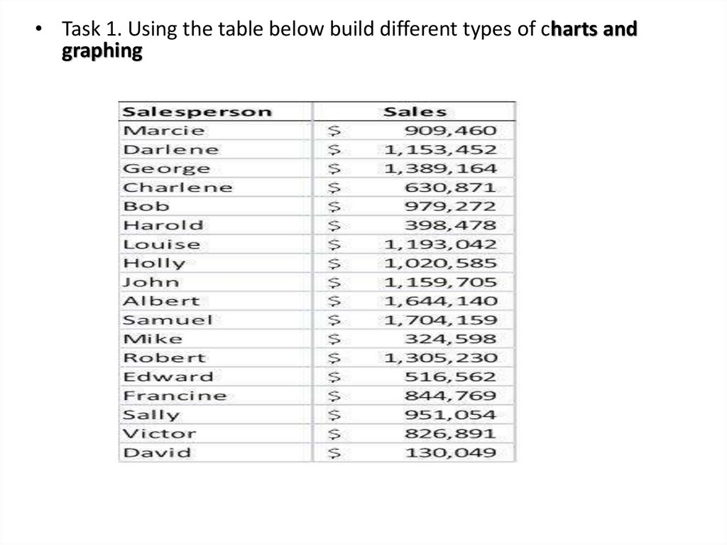
• Task 1. Using the table below build different types of charts and
graphing

26.

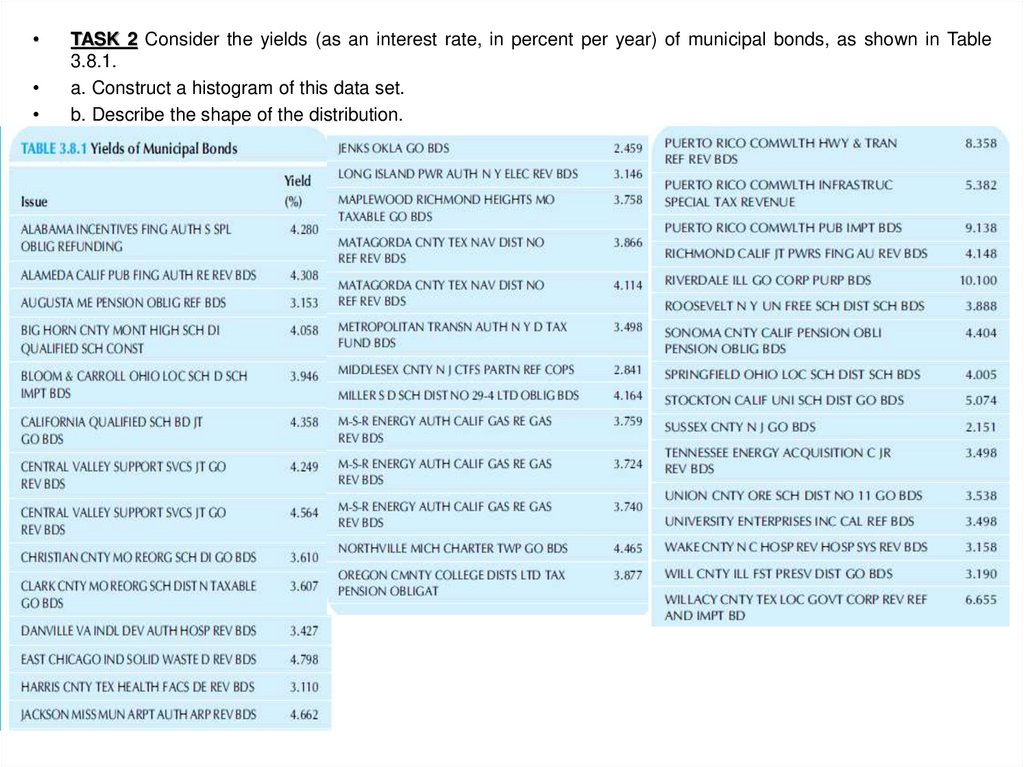
TASK 2 Consider the yields (as an interest rate, in percent per year) of municipal bonds, as shown in Table
3.8.1.
a. Construct a histogram of this data set.
b. Describe the shape of the distribution.

27. Landmark Summaries Interpreting Typical Values and Percentiles

• WHAT IS THE MOST TYPICAL VALUE?
There are three different ways to obtain such a
summary measure:
1. The average or mean, which can be computed
only for meaningful numbers (quantitative data).
2. The median, or halfway point, which can be
computed either for ordered categories (ordinal
data) or for numbers.
3. The mode, or most common category, which
can be computed for unordered categories
(nominal data), ordered categories, or numbers.

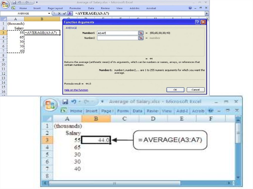
28. The Average: A Typical Value for Quantitative Data

• The average (also called the mean) is the most common method for
finding a typical value for a list of numbers, found by adding up all the
values and then dividing by the number of items. The sample average
expressed as a formula is:

29.

30. Excel’s Average function

31.

32.

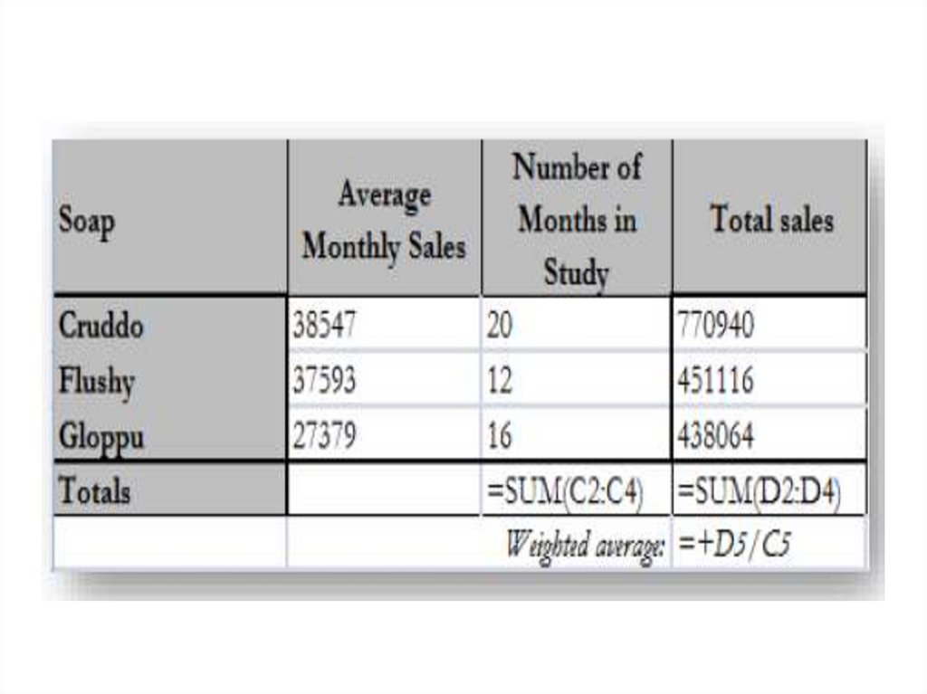
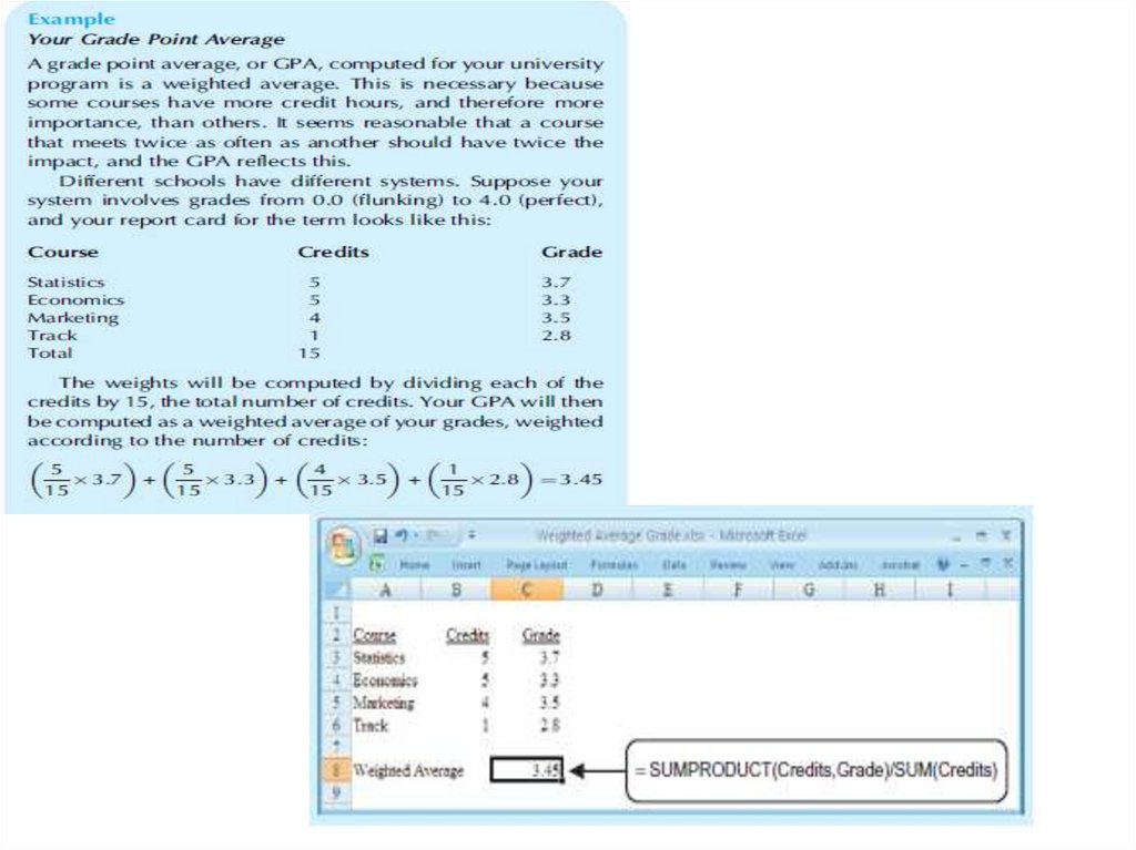
33. The Weighted Average: Adjusting for Importance

• The weighted average is like the average, except that it allows you to
give a different importance, or “weight,” to each data item. The
weighted average gives you the flexibility to define your own system of
importance when it is not appropriate to treat each item equally.

34.

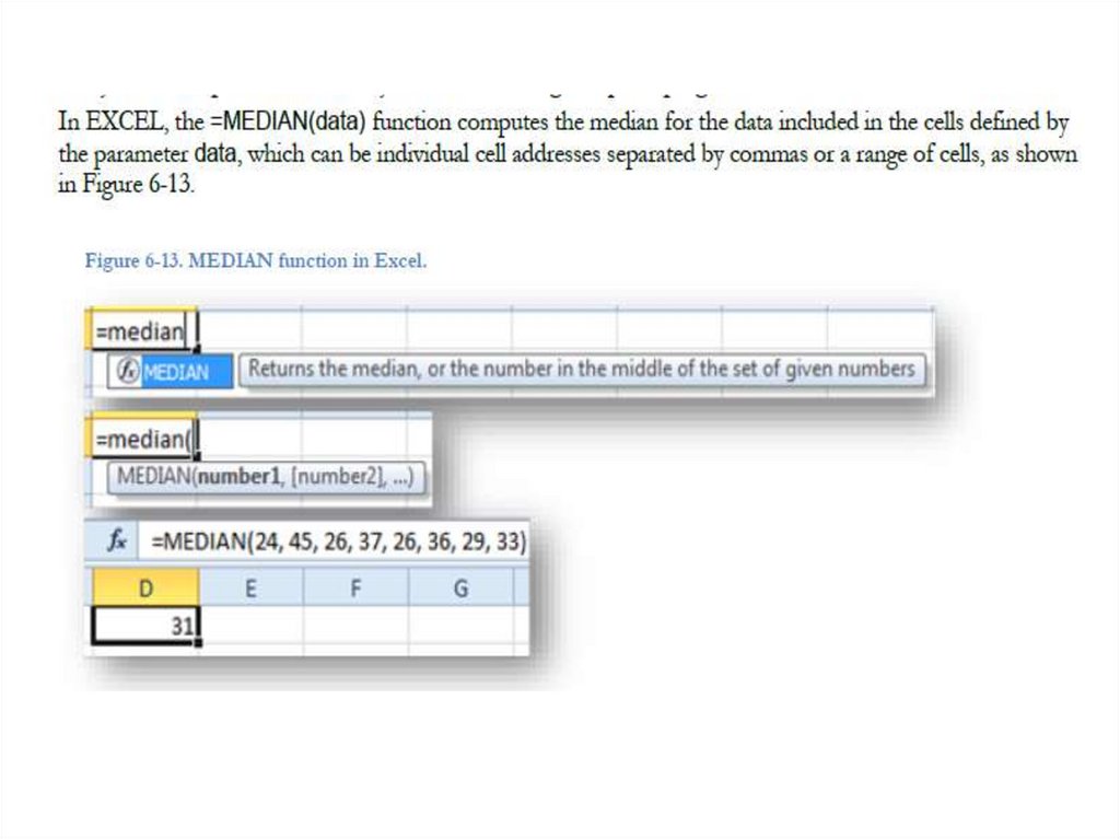
35. The Median: A Typical Value for Quantitative and Ordinal Data

• The median is the middle value; half of the items in the set are
larger and half are smaller. Thus, itmust be in the center of the
data and provide an effective summary of the list of data. You find
it by first putting the data in order and then locating the middle
value. To be precise, you have to pay attention to some details; for
example, you might have to average the two middle values if there
is no single value in the middle.
• One way to define the median is in terms of ranks. Ranks
associate the numbers 1, 2, 3,…,n with the data values so that the
smallest has rank 1, the next smallest has rank 2, and so forth up
to the largest, which has rank n.

36.

37.

38. The Mode: A Typical Value Even for Nominal Data

• The mode is the most common category, the one listed
most often in the data set. It is the only summary
measure available for nominal qualitative data because
unordered categories cannot be summed (as for the
average) and cannot be ranked (as for the median). The
mode is easily found for ordinal data by ignoring the
ordering of the categories and proceeding as if you had
a nominal data set with unordered categories.
• Mode is the value which occurs most frequently. The
mode may not exist, and even if it does, it may not be
unique.

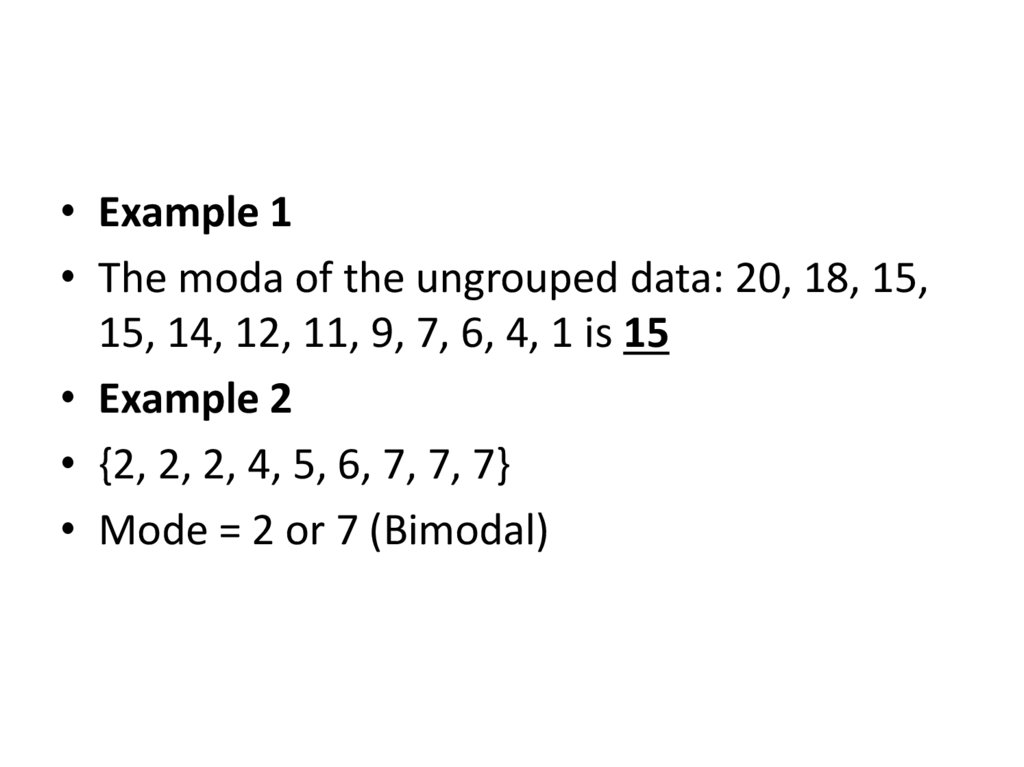
39.

• Example 1
• The moda of the ungrouped data: 20, 18, 15,
15, 14, 12, 11, 9, 7, 6, 4, 1 is 15
• Example 2
• {2, 2, 2, 4, 5, 6, 7, 7, 7}
• Mode = 2 or 7 (Bimodal)

40.

41. Task

To calculate:
The Average and The Weighted Average and Rang
1) 24, 26, 26, 29, 33, 36, 37
2) 24, 26, 26, 29, 33, 36, 37, 45
Median:
1) 37, 26, 29, 33, 24, 36, 26
2) 45, 26, 36, 29, 33, 37, 24, 26,
Moda
1) 24, 26, 26, 29, 33, 36, 37
2) 36, 26, 26, 29, 33, 36, 37, 45

42.

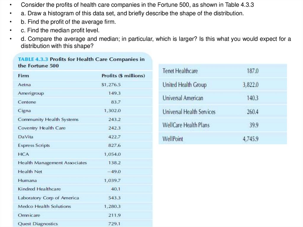
Consider the profits of health care companies in the Fortune 500, as shown in Table 4.3.3
a. Draw a histogram of this data set, and briefly describe the shape of the distribution.
b. Find the profit of the average firm.
c. Find the median profit level.
d. Compare the average and median; in particular, which is larger? Is this what you would expect for a
distribution with this shape?

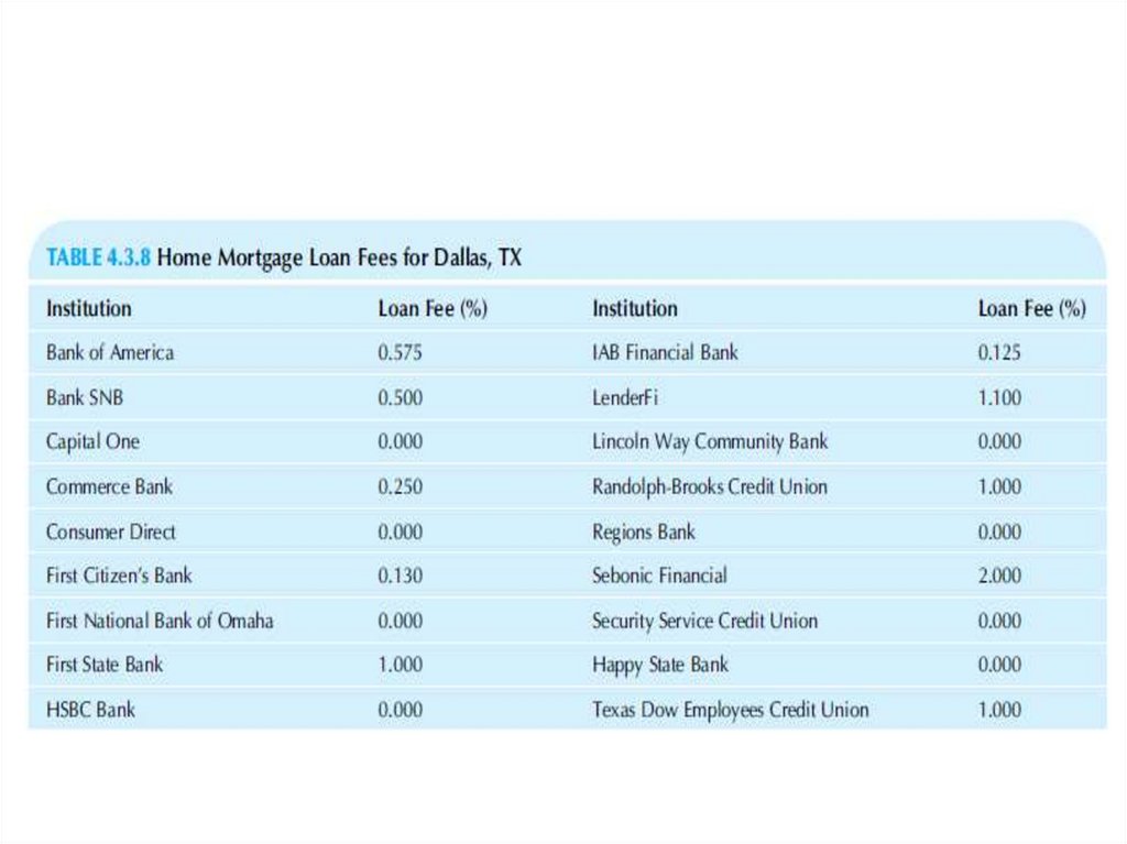
43. Task

• Consider the loan fees charged for granting home
mortgages,
• as shown in Table 4.3.8, for Dallas TX, 30-year fixed rate for
home purchase, with credit Score 740+, and with 20%
down payment. These are given as a percentage of the loan
amount and are one-time fees paid when the loan is
closed.
• a. Find the average loan fee.
• b. Find the median loan fee.
• c. Find the mode.
• d. Which summary is most useful as a description of the
“typical” loan fee, the average, median, or mode? Why?

44.

45. Probability Understanding Random Situations

• Probability is a measure quantifying the likelihood that events will
occur.
• Probability. How likely something is to happen. Many events can't
be predicted with total certainty.
• If events are mutually incompatible (they can’t occure at the same
time) and they constitute all possibilities for a given situation, the
sum of their individual probabilities is one. For example, a fair
cubical die has a probability
pi = 1/6
• of landing with the top face showing one dot (i=1) facing up;
indeed pi = 1/6 for all i. The probability that a fair die will land
showing a top face of either a 1 or a 2 or a 3 or a 4 or a 5 or a 6 is
• Σpi = 1

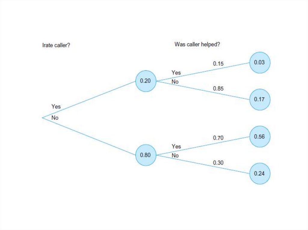
46.

• A probability tree is a picture indicating
probabilities and conditional probabilities for
combinations of two or more events. We will
begin with an example of a completed tree
and follow up with the details of how to
construct the tree.
• Probability trees are closely related to decision
trees, which are used in finance and other
fields in business.