Empirical tools

1. Empirical tools (recap):

Determination of statistical regularities (correlation).
Determination of causality.
Control vs Treatment groups.
Differences-in-differences estimates.
Experimentation and simulation.
Structural models.
….

2. THE IMPORTANT DISTINCTION BETWEEN CORRELATION AND CAUSATION

There are many examples where causation and
correlation get confused.
It is critical for government policy to understand the
difference; otherwise policy may not have the
intended impact.

3. THE IMPORTANT DISTINCTION BETWEEN CORRELATION AND CAUSATION

One interesting example is about Russian peasants.
There was a cholera epidemic. Government sent
doctors to the worst-affected areas to help.
Peasants observed that in areas with lots of doctors,
there was lots of cholera.
Peasants concluded doctors were making things
worse.
Based on this insight, they murdered the doctors.

4. THE IMPORTANT DISTINCTION BETWEEN CORRELATION AND CAUSATION

Another example concerns SAT preparation
courses.
In 1988, Harvard interviewed its freshmen and found
those who took SAT “coaching” courses scored 63
points lower than those who did not.
One dean concluded that the SAT courses were
unhelpful and “the coaching industry is playing on
parental anxiety.”

5. The Problem

In both examples, there is a common problem: an
attempt to interpret a correlation as a causal relationship,
without sufficient thought to the underlying data
generating process.
For any correlation between two variables A and B,
there are three possible explanations for a
correlation:
A is causing B.
B is causing A.
Some other factor is causing both.

6. The Problem

In the Russian peasant example, the possibilities
might be:
Doctors cause peasants to die from cholera through
incompetent treatment.
Higher incidence of illness caused more physicians to
be present.
Peasants thought the first possibility was correct.

7. The Problem

In the Harvard SAT example, the possibilities could
be:
SAT prep courses worsen preparation for the SATs.
Those with poorer test taking ability take prep
courses to try to catch up.
Those who are generally nervous both like to take
prep courses and do the worst on standardized
exams.
Harvard dean thought the first possibility was
correct.

8. MEASURING CAUSATION WITH DATA WE’D LIKE TO HAVE: RANDOMIZED TRIALS

The “gold standard” of causality is a randomized trial.
The trial proceeds by taking a group of volunteers and
randomly assigning them to either a “treatment” group that
gets the intervention, or a “control” group that is denied
the intervention.
With random assignment, the assignment of the intervention
is not determined by anything about the subjects.
As a result, the treatment group is identical to the control
group in every facet but one: the treatment group gets the
intervention.

9. Control vs Treatment groups. Randomness vs Biases.

In the SAT example, the “treatment” group
members are those who took the coaching course;
the “control” group members are those who did
not.
In the Russian peasant example, the “treatment”
group were communities where doctors were
assigned, the “control” group were communities
where doctors were not assigned.
Immediate test (key intuition):
Do the treatment and control groups differ for any
reason other than the treatment?

10. Randomized Trials in the TANF Context

Imagine a large group (say, 2000) of single mothers
were randomly assigned to one of two groups with a
coin flip:
The “control” group continues to receive a guarantee
of $5,000.
The “treatment” group now has their TANF benefit
cut to $3,000.
Follow groups for a period of time, and measure the
work effort.

11. Randomized Trials in the TANF Context

In an experiment like this in California in 1992, the
elasticity of employment with respect to welfare
benefits was estimated to be -0.67.
Thus, a 10% decrease in benefits resulted in a 6.7%
increase in employment.

12. Why We Need to Go Beyond Randomized Trials

Randomized trials present some problems:
They can be expensive.
They can take a long time to complete.
They may raise ethical issues (especially in the context of
medical treatments).
Parkinson’s disease treatment.
The inferences from them may not generalize to the
population as a whole.
Subjects may drop out of the experiment for non-random
reasons, a problem known as attrition.
For these reasons (especially the first one about randomized
trials being expensive), economists often take different
approaches to try to assess causal relationships in empirical
research.

13. ESTIMATING CAUSATION WITH THE DATA WE ACTUALLY GET: OBSERVATIONAL DATA

There are four main approaches:
Time series analysis
Cross-sectional regression analysis
Quasi-experiments
Structural modeling

14.

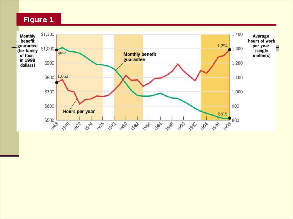
Figure 1

15. Time Series Analysis

Figure 1 reveals that real benefits have declined dramatically
over time, while average hours have risen substantially.
Apparently supports the theory that TANF benefit cuts
should increase labor supply.
There are problems, however.
Two sub-periods (1968-1976, and 1978-1983) show negative
effect on labor supply, or zero effect.
Highlights difficulty that when there is a slow moving trend
(benefit declines), it is very difficult to infer causal effect of
this on another variable.

16. Time Series Analysis

Many potential explanations for the changes, too,
such as:
Greater acceptance of women in workplace.
Better child care options.
Changes in social norms about working.
Other government program like the earned income
tax credit.
Economic growth.

17. Quasi-Experiments

Quasi-experiments are changes in the economic
environment that create roughly identical treatment and
control groups for studying the effect of that environmental
change.
This allows researchers to take advantage of randomization
created by external forces.
Basic approach is to let outside forces do the randomization
for us. In some cases, the situation happens naturally.
Suppose, for example, that Arkansas cut its TANF benefit by
20% in 1997, and that we had a large sample of single mothers
in Arkansas in 1996 and 1998.
At the same time, imagine that Louisiana’s benefits remained
unchanged.

18. Quasi-Experiments

In principle, the alteration in the states’ policies has
essentially performed our randomization for us.
The women in Arkansas who experienced the
decrease in benefits are the treatment group.
The women in Louisiana whose benefits were
unchanged are the control.
By computing the change in labor supply across
these groups, and then examining the difference
between treatment (Arkansas) and control
(Louisiana), we can obtain an estimate of the impact
of benefits on labor supply that is free from bias.

19. Quasi-Experiments

Imagine we simply studied single mothers in
Arkansas alone.
Arkansas has essentially performed an “experiment”
where single mothers in 1996 are the control group,
and those in 1998 are the treatment group.
In practice, this comparison runs into the criticisms
that confront us with time series analysis.
For example, the national economy was growing
exceptionally fast during this period.

20. Quasi-Experiments

Because of these concerns about national trends, the
quasi-experimental approach includes the extra step
of comparing the treatment group for whom the
policy changed to a control group for whom it did
not.
Single mothers in Louisiana did not experience the
TANF cut, yet benefited from the growth in the
economy.

21. Quasi-Experiments

That is, by examining hours of work in Arkansas, we
obtain:
HOURSAR,1998-HOURSAR,1996
This contains both the treatment effect and the bias
from the economic boom.
In contrast, by examining hours of work in
Louisiana, we obtain:
HOURSLA,1998-HOURSLA,1996
This contains only the effect of the economic boom.

22. Quasi-Experiments

By subtracting the change in hours of work in
Louisiana from that in Arkansas, we control for the
bias caused by the economic boom.
We obtain a causal estimate of the effect of TANF
benefits on hours of work.
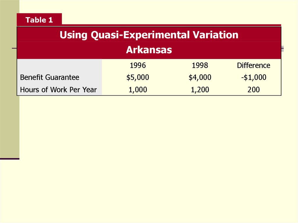
An example is given in Table 1, first focusing on
Arkansas alone.

23.

Table 1
Using Quasi-Experimental Variation
Arkansas
1996
1998
Difference
Benefit Guarantee
$5,000
$4,000
-$1,000
Hours of Work Per Year
1,000
1,200
200

24. Quasi-Experiments

While benefits fell by 20%, hours of work increased
by 20%; the implied elasticity of labor supply with
respect to benefits levels is -1.
This is larger than the -0.67 elasticity estimate found
in the randomized trial in California.

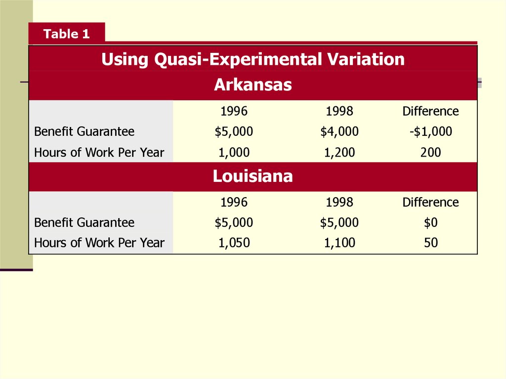
25. Quasi-Experiments

There is likely to be bias in this “first-difference,”
because there was major economic growth during
this period.
Thus, single mothers in Arkansas may have increased
their work effort even if TANF benefits had not
fallen.
We examine single mothers in the neighboring state
of Louisiana, in the bottom panel of Table 1.

26.

Table 1
Using Quasi-Experimental Variation
Arkansas
1996
1998
Difference
Benefit Guarantee
$5,000
$4,000
-$1,000
Hours of Work Per Year
1,000
1,200
200
1996
1998
Difference
Benefit Guarantee
$5,000
$5,000
$0
Hours of Work Per Year
1,050
1,100
50
Louisiana

27. Quasi-Experiments

This approach yields the difference-in-difference
estimator – the difference between the changes in
outcomes for the treatment group that experiences
an intervention and a control group that does not.
We are taking the difference in labor supply changes
in these states in an attempt to purge the estimate of
bias (due to the growing economy).
While cross-sectional analysis would suggest that the
reduction in welfare benefits leads to a 100-hour
increase in work, the difference-in-difference analysis
suggests a 150-hour increase.

28. Quasi-Experiments

The difference-in-difference estimator is:
HOURS
AK ,1998
HOURS AK ,1996 HOURS LA,1998 HOURS LA,1996
The second term, for Louisiana, nets out the bias
from the growing economy.
Thus, the causal effect of TANF benefit cuts would
be a 150-hour increase in labor supply.

29. Quasi-Experiments: Problems with quasi-experimental analysis

This approach also has problems, however.
It is possible that the economic boom affected
Arkansas differently than it did Louisiana.
More generally, single mothers may be different
across states.
We can never be completely certain that we have
purged the treatment-control comparisons of bias.

30. Recap: trials of ERT

ERT is the estrogen replacement therapy, which is a popular
treatment for women who have gone through menopause.
Menopause is associated with many negative side effects.
ERT reduces those by mimicking the estrogen produced
before the onset of menopause.
Concern about ERT: Does it raise the risk of heart disease?
A series of studies (from 1980s) compared women who did
and did not underwent ERT.
They found no higher risk, and, in fact, if anything, ERT
lowered the risk of heart attacks.
Do you see the problem?

31. Trials of ERT. The problem.

Women who underwent ERT are more likely to be under a
doctor’s care, lead healthier lifestyle, have more income: all
of these are associated with a lower chance of heart
problems.
Randomizes trials of ERT.
1991. National Institute of Health appoints its first female
director, Dr. B. Healy. She sponsors a randomized trial of
ERT.
16000 women ages 50-79 participate.
Supposed to last 8.5 years, stopped after 5.2.
ERT did raise the risk of hart disease (and of invasive breast
cancer).
Lead to more careful recommendations.