


 economics
Similar presentations:


Supply 11.2a
1. Supply 11.2a
03/09/2018Sonali Sinha Roy
1
2. Learning Objectives
By the end of the lesson the learners will be able to :Define and understand the terms
Supply
Movement along and shift in the Supply curves
Analyse and apply the concept to real world situation .
(1 min)
3. Willingness to sell product at various given prices at a given point of time
03/09/2018Sonali Sinha Roy
3
4. Supply Curve
03/09/2018Sonali Sinha Roy
4
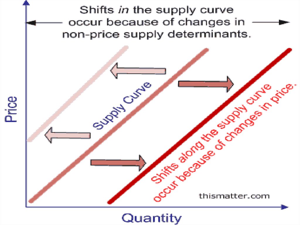
5. Movement along the Supply Curve
Movement along the Supply curve isdue to the change in price only.
Other factors are kept constant .
Movement from Point A to B:
Extension in Supply/Increase in
Quantity Supplied - P ↑ QD ↑
Movement from Point C to B:
Contraction in Supply/Decrease in
Quantity Supplied - P ↓ QD ↓
03/09/2018
Sonali Sinha Roy
5
6.
03/09/2018Sonali Sinha Roy
6
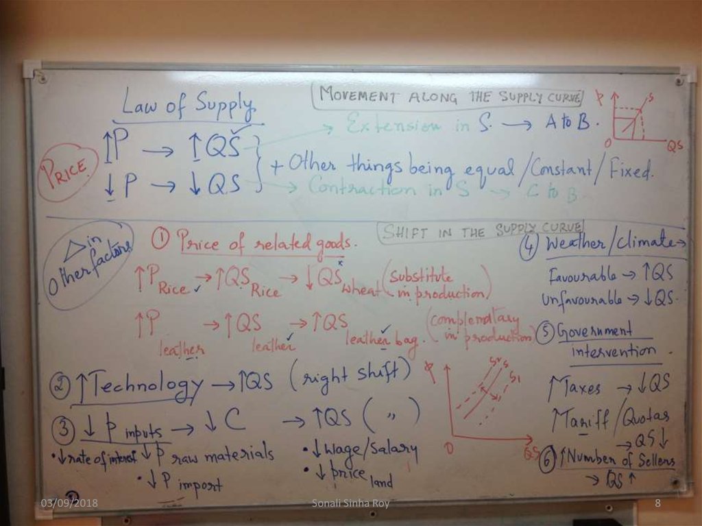
7. Shifts in supply curve
SPENTS = Supplier prices (FOP)
P = Price of related goods
E = Expected price in future
N = Number of sellers
4Ts= Tax
Technology
Temperature
Tampering
03/09/2018
Sonali Sinha Roy
7
8.
03/09/2018Sonali Sinha Roy
8
9.
03/09/2018Sonali Sinha Roy
9
10. Supply curve shifts to the right
Why might the supplycurve shift to the right?
•Fall in wage costs
•Fall in raw material costs
•Improved labour productivity
•Reduced indirect taxes
•Increased subsidies
•Improved technology
•Entry of new firms into the
industry
Initial equilibrium: P1, Q1 (A)
New equilibrium: P4, Q6 (G)
03/09/2018
Sonali Sinha Roy
10
11. Supply curve shifts to the left
Why might the supplycurve shift to the left?
•Rise in wage costs
•Rise in raw material costs
•Reduced labour productivity
•An increase in indirect taxes
•Reduced, or elimination of,
subsidies
•The exit of existing firms
from the industry
Initial equilibrium: P1, Q1 (A)
New equilibrium: P5, Q8 (J)
03/09/2018
Sonali Sinha Roy
11
12. Example: Case Study
03/09/2018Sonali Sinha Roy
12
13. Recap of Today’s Lesson
03/09/2018Sonali Sinha Roy
13
14. Reflection
03/09/2018Sonali Sinha Roy
14
15. Supply 11.2a
03/09/2018Sonali Sinha Roy
15
16. Learning Objectives
By the end of the lesson the learners will be able to :Define and understand the terms
Supply Function
Plot supply curve from an given equation
Analyse and apply the concept to real world situation .
(1 min)
17. Supply Function
Supply Function indicates the relationshipbetween the of the quantity commodity
supplied and the unit price of the commodity.
Equation:
Qs = c + dP
Qs = quantity of a good supplied
P = is the price of the good
c = vertical intercept (max supply)
d = the slope of the supply curve
03/09/2018
Sonali Sinha Roy
17
18. Supply Function
c = Autonomous level of supply (how muchwould be produced if the price is zero)-vertical
intercept
d = the price coefficient of supply (how much
quantity will increase for every $1 increase in
price. Higher the d variable, higher the producer
responsive to the price change and vice versa) the slope of the supply curve
03/09/2018
Sonali Sinha Roy
18
19. Example
03/09/2018Sonali Sinha Roy
19
20. Supply Function
The slope of a supply curve is usually positive ,as price increases, quantity supplied increases
and vice-versa.
The y-intercept of the supply curve (0,b)
represents the lowest price at which an item
will be supplied.
03/09/2018
Sonali Sinha Roy
20
21. In Class Activity
Use the linear supply equation for haircuts in your town, Qs=-100+20P to answer thequestions that follow:
1.Create a schedule showing the supply of haircuts in your town at prices of $10, $20,
$30, $40, and $50.
2.Calculate the price-intercept of your supply curve, and then use the data from your
supply schedule to plot a supply curve for haircuts.
3.Assume that due to a decrease in rents on business space in your town, the number
of salons increases, increasing the ‘c’ variable in your supply equation to -50. Create a
new supply schedule based on the new supply equation, and then plot your new
supply curve on your graph.
4.Assume due to a change in labor laws, it becomes more difficult for salons to hire
and fire hair stylists, reducing the responsiveness of salons to changes in the price of
haircuts. This leads to a fall in the‘d’ variable in the supply equation to 10. Create a
new supply schedule based on the new supply equation, and then plot your new
supply curve on your graph.
5.Besides the two non-price factors described above, identify at least five other factors
that can lead to a change in the supply of haircuts or a change in the responsiveness of
salons to price changes.
03/09/2018
Sonali Sinha Roy
21
22. Recap of Today’s Lesson
03/09/2018Sonali Sinha Roy
22
23. Reflection
03/09/2018Sonali Sinha Roy
23