How Competition Shapes the Creation and Distribution of Economic Value

1. How Competition Shapes the Creation and Distribution of Economic Value

Introduction to Business Strategy
Prof. Marvin Lieberman
UCLA Anderson School of Management
How Competition Shapes the
Creation and Distribution
of Economic Value
Lecture 2: Porter’s Five Forces
©2009 by Marvin Lieberman

2.

Michael Porter’s “Five Forces of Competition”
framework describes how the structural features
of an industry influence the distribution of value
created by firms within that industry.
Ideally, firms in an industry would like to capture
most or all of the economic value that they create.
However, competitive forces operate to push that
value “forward” to customers (in the form of lower
prices), or in some cases, “backward” to suppliers.
*Michael E. Porter (1980). Competitive Strategy. Free Press, Boston.
©2009 by Marvin Lieberman

3.

Michael Porter developed his Five Forces
concept from basic ideas in the field of
industrial economics. In this set of lectures,
we will see how these economic forces
operate.
©2009 by Marvin Lieberman

4.

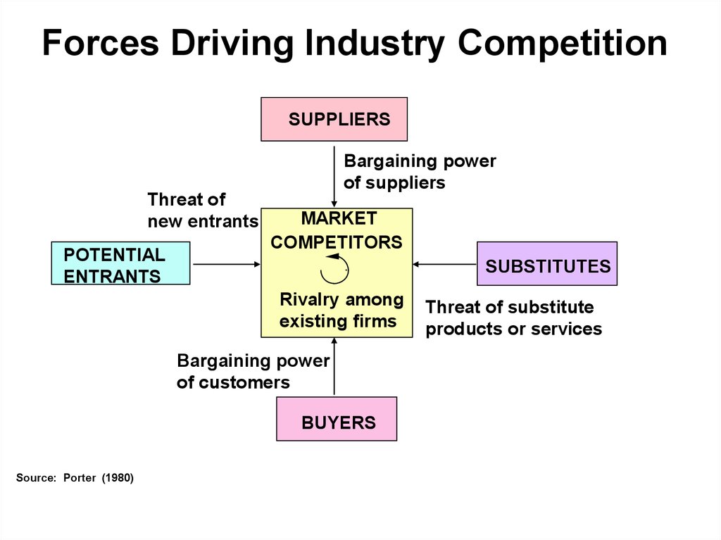
Forces Driving Industry Competition
SUPPLIERS
4. Bargaining power
of suppliers
3. Threat of
new entrants
POTENTIAL
ENTRANTS
MARKET
COMPETITORS
SUBSTITUTES
2. Rivalry among
existing firms
1. Bargaining power
of customers
BUYERS
Source: Porter (1980)
5. Threat of substitute
products or services

5.

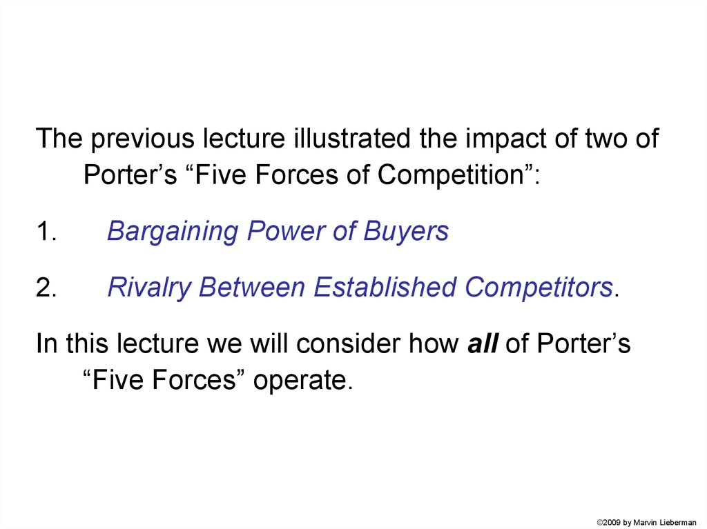
The previous lecture illustrated the impact of two of
Porter’s “Five Forces of Competition”:
1.
Bargaining Power of Buyers
2.
Rivalry Between Established Competitors.
In this lecture we will consider how all of Porter’s
“Five Forces” operate.
©2009 by Marvin Lieberman

6.

Let’s begin with the two forces implicit in the
examples from last time.
According to Porter (1980), the bargaining power of
buyers depends on buyer concentration,
information, and other factors.
Consider Examples 1.1 and 1.2 from the last lecture.
©2009 by Marvin Lieberman

7.

Example 1.1
One firm able to produce one unit of “product” at cost=0.
F1
B1
One buyer, able to consume one unit of “product,” and willing to pay $1.
High buyer concentration gives B1 bargaining power.
(In this example of “bilateral monopoly” F1 also has power.)
• What will be the price (P) of the “product”?
0<P≤1
• How much value (V) is created?
V=1
• Who captures that value?
“pure bargaining” case
©2009 by Marvin Lieberman

8.

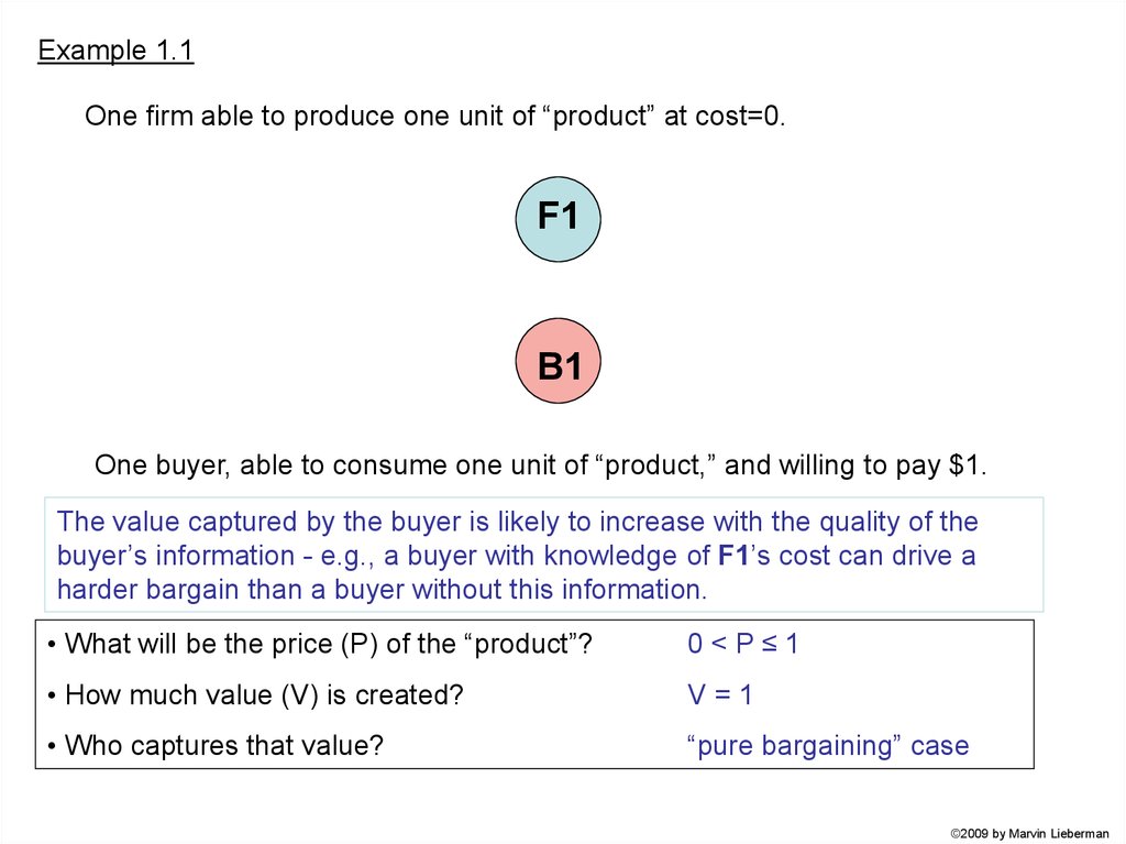
Example 1.1
One firm able to produce one unit of “product” at cost=0.
F1
B1
One buyer, able to consume one unit of “product,” and willing to pay $1.
The value captured by the buyer is likely to increase with the quality of the
buyer’s information - e.g., a buyer with knowledge of F1’s cost can drive a
harder bargain than a buyer without this information.
• What will be the price (P) of the “product”?
0<P≤1
• How much value (V) is created?
V=1
• Who captures that value?
“pure bargaining” case
©2009 by Marvin Lieberman

9.

Example 1.2
One firm able to produce one unit of “product” at cost=0.
F1
B1
B2
Two buyers, each able to consume one unit of product and willing to pay up to $1.
Competition among buyers reduces their bargaining power.
• What will be the price of the “product”?
P = 1 (increase from Ex.1)
• How much value is created?
V=1
• Who captures that value?
“simple monopoly” case
(F1 captures all value)
©2009 by Marvin Lieberman

10. Buyer power greater when:

Implications
Buyer power greater when:
• Buyers are more concentrated
• Buyers are better informed
©2009 by Marvin Lieberman

11.

We also saw that an increase in producer rivalry
makes the industry less attractive.
Consider examples 1.5 and 1.6.
©2009 by Marvin Lieberman

12.

Example 1.6
F1 can produce unlimited quantity at cost=0.
F1
c=0
B1
B2
B3
B4
B5
wtp=1.0
wtp=0.8
wtp=0.6
wtp=0.4
wtp=0.2
Units
Price
TR
MR
1
1.0
1.0
1.0
2
0.8
1.6
0.6
3
0.6
1.8
0.2
4
0.4
1.6
-0.2
5
0.2
1.0
-0.6
F1 is a monopolist, so there is no industry rivalry.
• What will be the price of the “product”?
P = 0.6
• How much value is created?
V = 2.4
• Who captures that value?
F gets 1.8
B1 gets 0.4
B2 gets 0.2
B3 gets zero
(= 1.0 + 0.8 + 0.6)
©2009 by Marvin Lieberman

13.

Example 1.7
F1 and F2 have unit cost=0. Neither is output constrained.
F1
F2
c=0
c=0
B1
B2
B3
B4
B5
wtp=1.0
wtp=0.8
wtp=0.6
wtp=0.4
wtp=0.2
As producer concentration falls, rivalry increases.
• What will be the price of the “product”?
P = 0 (“Bertrand” competition)
• How much value is created?
V = 3.0
• Who captures that value?
F1 and F2 get zero
B1 gets 1.0
B2 gets 0.8
etc.
(= 1 + .8 + .6 + .4 + .2)
©2009 by Marvin Lieberman

14.

Example 1.7
F1 and F2 have unit cost=0. Neither is output constrained.
F1
F2
c=0
c=0
B1
B2
B3
B4
B5
wtp=1.0
wtp=0.8
wtp=0.6
wtp=0.4
wtp=0.2
Note that if the producers had limited capacity they would capture value.
Industry “excess capacity” reduces their bargaining power.
• What will be the price of the “product”?
P = 0 (“Bertrand” competition)
• How much value is created?
V = 3.0
• Who captures that value?
F1 and F2 get zero
B1 gets 1.0
B2 gets 0.8
etc.
(= 1 + .8 + .6 + .4 + .2)
©2009 by Marvin Lieberman

15.

Example 1.7
F1 and F2 have unit cost=0. Neither is output constrained.
F1
F2
c=0
c=0
Exit
Barriers
B1
B2
B3
B4
B5
wtp=1.0
wtp=0.8
wtp=0.6
wtp=0.4
wtp=0.2
If one producer exited, the other would be profitable. In an industry with
excess capacity, exit barriers prolong the period of depressed profitability.
• What will be the price of the “product”?
P = 0 (“Bertrand” competition)
• How much value is created?
V = 3.0
• Who captures that value?
F1 and F2 get zero
B1 gets 1.0
B2 gets 0.8
etc.
(= 1 + .8 + .6 + .4 + .2)
©2009 by Marvin Lieberman

16. Implications

Rivalry increases with:
• More direct competitors
• Industry excess capacity
• Exit barriers
©2009 by Marvin Lieberman

17.

Now let’s consider the threat of entry.
©2009 by Marvin Lieberman

18.

Example 1.7
F1 and F2 have unit cost=0. Neither is capacity constrained.
F1
F2
c=0
c=0
B1
B2
B3
B4
B5
wtp=1.0
wtp=0.8
wtp=0.6
wtp=0.4
wtp=0.2
In this example, F1 and F2 are rival producers in the industry.
What happens if F2 is only a potential entrant to the industry?
©2009 by Marvin Lieberman

19.

Example 1.7a
F1 and F2 have unit cost=0. Neither is capacity constrained.
F1
F2
c=0
c=0
B1
B2
B3
B4
B5
wtp=1.0
wtp=0.8
wtp=0.6
wtp=0.4
wtp=0.2
If F2 can enter very quickly, price falls to the same level
as when F1 and F2 are direct competitors.
The threat of entry may be enough to force F1 to charge
a low price, even if F2 does not actually enter.
©2009 by Marvin Lieberman

20.

Example 1.7b
F1 and F2 have unit cost=0. Neither is capacity constrained.
F1
F2
c=0
c=0
B1
B2
B3
B4
B5
wtp=1.0
wtp=0.8
wtp=0.6
wtp=0.4
wtp=0.2
If entry takes a long time, F1 may be able to charge a
relatively high price, at least initially.
©2009 by Marvin Lieberman

21.

Example 1.7c
F2 has higher cost. Neither firm is capacity constrained.
F1
c=0
B1
B2
B3
B4
B5
wtp=1.0
wtp=0.8
wtp=0.6
wtp=0.4
wtp=0.2
$
$
$
$
$
$
$
$
F2
c=.5
If entry involves substantial fixed (sunk) costs, or if
potential entrants are less efficient, F1 may be able to
deter them by pricing moderately or by threatening price
cuts following entry.
If the “entry barriers” are high enough, no entry will occur
regardless of actions by F1.
©2009 by Marvin Lieberman

22. Potential Entrants

Implications
Potential Entrants
• Almost like rival producers (when entry is fast)
• Impeded by “entry barriers” (costs of entry)
• Incumbents can take actions to deter entry
©2009 by Marvin Lieberman

23.

Now let’s consider the impact of “supplier power.”
We will add supplier(s) as an additional level of potential value creation,
beyond the firm-buyer interactions we have been considering so far.
Adding suppliers as a second stage creates a simple “value chain”.
©2009 by Marvin Lieberman

24.

New Example.
F1 and F2 have cost=0 and each can produce one unit.
B1, B2 and B3 each can consume one unit and have WTP=1.
F1
F2
c=0
c=0
B1
B2
B3
wtp=1
wtp=1
wtp=1
What is the product price?
Who captures the value?
P=1
All value distributed to F1 and F2.
©2009 by Marvin Lieberman

25.

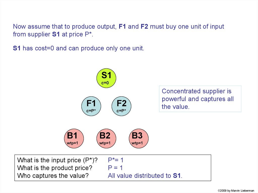
Now assume that to produce output, F1 and F2 must buy one unit of input
from supplier S1 at price P*.
S1 has cost=0 and can produce only one unit.
S1
c=0
F1
F2
c=P*
c=P*
Concentrated supplier is
powerful and captures all
the value.
B1
B2
B3
wtp=1
wtp=1
wtp=1
What is the input price (P*)?
What is the product price?
Who captures the value?
P*= 1
P=1
All value distributed to S1.
©2009 by Marvin Lieberman

26.

Now let’s add additional suppliers.
F1 and F2 must buy one unit of input from a supplier.
S1, S2 and S3 have cost=0, and each can produce one unit.
S1
S2
S3
c=0
c=0
c=0
F1
F2
c=P*
c=P*
B1
B2
B3
wtp=1
wtp=1
wtp=1
What is the input price?
What is the product price?
Who captures the value?
P*= 0
P=1
All value distributed to F1 and F2.
©2009 by Marvin Lieberman

27. Implications

Supplier Power
• Suppliers can siphon value from producers
• Power increases with supplier concentration
• Analysis similar to buyer power
• Important issue: At what stage(s) are profits
captured within the industry “value chain”?
©2009 by Marvin Lieberman

28. Application

One example of a supplier with market power is Microsoft, whose “Windows”
software has long maintained a dominant share of the PC operating system market.
Microsoft’s position approaches that of a single supplier selling to a large number of
PC manufacturers. Not surprisingly, Microsoft enjoys high margins and captures a
large share of total profits within the PC industry value chain.
Microsoft does face competitors who also supply computer operating systems, but
typically the alternatives to Microsoft Windows are not close substitutes. If a close
substitute for Windows emerged at a low price, surely it would threaten Microsoft’s
margins. In general, the intensity of competition facing firms in an industry – or
facing a specific firm like Microsoft with a “differentiated product” – depends on the
closeness of substitute products. We now turn to the “threat of substitutes,” the last
and most subtle of Porter’s five forces.
©2009 by Marvin Lieberman

29.

As we will see, substitutes act to reduce the economic value
that firms in the focal industry can create. In general, the
incremental value created by a given product will diminish as
the substitute product becomes cheaper or better in quality.
©2009 by Marvin Lieberman

30.

As we will see, substitutes act to reduce the economic value
that firms in the focal industry can create. In general, the
incremental value created by a given product will diminish as
the substitute product becomes cheaper or better in quality.
Let’s start by elaborating the case we saw in the first lecture,
in Example 1.1.
If you find it helpful to think in terms of specific examples, imagine that the
“product” in this example is Apple’s iPod, which we will assume exists in a
unique industry by itself. The iPod faces a “substitute” industry, which
consists of the set of competing MP3 players. We will start with a base case
where the iPod has the entire field to itself without any substitutes. Then,
we will introduce MP3 substitutes of poor quality compared to the iPod.
Finally, we will see what happens when we improve the substitute’s quality
and/or reduce its price.
©2009 by Marvin Lieberman

31.

Example 1.1
One firm able to produce one unit of “product” at cost=0.
F1
B1
One buyer, able to consume one unit of “product,” and willing to pay $1.
Consider this example in the context of the iPod: In the absence of any substitute, Apple can charge
any price up to $1, and the buyer will purchase the iPod. The availability of the iPod creates $1 of
value in this case.
• What is the most B1 is willing to pay for “product”?
WTP = V = 1
• What will be the price of the “product”?
0<P≤1
• Range of potential profit to F1?
0
1
©2009 by Marvin Lieberman

32.

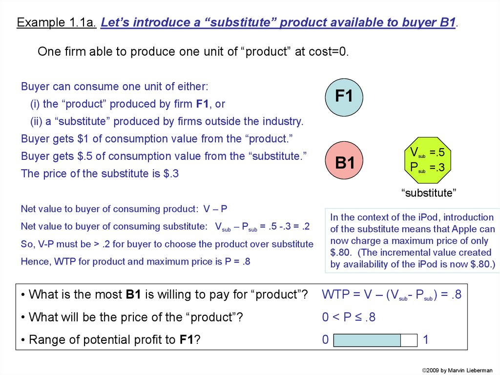
Example 1.1a. Let’s introduce a “substitute” product available to buyer B1.
One firm able to produce one unit of “product” at cost=0.
Buyer can consume one unit of either:
F1
(i) the “product” produced by firm F1, or
(ii) a “substitute” produced by firms outside the industry.
Buyer gets $1 of consumption value from the “product.”
Buyer gets $.5 of consumption value from the “substitute.”
B1
The price of the substitute is $.3
V =.5
P =.3
sub
sub
“substitute”
Net value to buyer of consuming product: V – P
In the context of the iPod, introduction
of the substitute means that Apple can
now charge a maximum price of only
$.80. (The incremental value created
by availability of the iPod is now $.80.)
Net value to buyer of consuming substitute: Vsub – Psub = .5 -.3 = .2
So, V-P must be > .2 for buyer to choose the product over substitute
Hence, WTP for product and maximum price is P = .8
• What is the most B1 is willing to pay for “product”?
WTP = V – (Vsub- Psub) = .8
• What will be the price of the “product”?
0 < P ≤ .8
• Range of potential profit to F1?
0
1
©2009 by Marvin Lieberman

33.

Example 1.1b. Let’s reduce the price of the substitute product.
One firm able to produce one unit of “product” at cost=0.
Buyer can consume one unit of either:
F1
(i) the “product” produced by firm F1, or
(ii) a “substitute” produced by firms outside the industry.
Buyer gets $1 of consumption value from the “product.”
Buyer gets $.5 of consumption value from the “substitute.”
B1
The price of the substitute is $.1
V =.5
P =.1
sub
sub
Substitute
product
Net value to buyer of consuming product: V – P
In the context of the iPod, the price cut
of the substitute means that Apple can
So, V-P must be > .4 for buyer to choose the product over substitute now charge a maximum price of only
$.60. (The incremental value created by
Hence, WTP for product and maximum price is P = .6
availability of the iPod is now $.60.)
Net value to buyer of consuming substitute: Vsub – Psub = .5 -.1 = .4
• What is the most B1 is willing to pay for “product”?
WTP = V – (Vsub- Psub) = .6
• What will be the price of the “product”?
0 < P ≤ .6
• Range of potential profit to F1?
0
1
©2009 by Marvin Lieberman

34.

Example 1.1c. Now, let’s improve the “quality” of the substitute product.
One firm able to produce one unit of “product” at cost=0.
Buyer can consume one unit of either:
F1
(i) the “product” produced by firm F1, or
(ii) a “substitute” produced by firms outside the industry.
Buyer gets $1 of consumption value from the “product.”
Buyer gets $.9 of consumption value from the “substitute.”
B1
The price of the substitute is $.1
V =.9
P =.1
sub
sub
Substitute
product
Net value to buyer of consuming product: V – P
In the context of the iPod, improvement
of the substitute means that Apple can
So, V-P must be > .8 for buyer to choose the product over substitute now charge a maximum price of only
$.20. (The incremental value created by
Hence, WTP for product and maximum price is P = .2
availability of the iPod is now only $.20.)
Net value to buyer of consuming substitute: Vsub – Psub = .9 -.1 = .8
• What is the most B1 is willing to pay for “product”?
WTP = V – (Vsub- Psub) = .2
• What will be the price of the “product”?
0 < P ≤ .2
• Range of potential profit to F1?
0
1
©2009 by Marvin Lieberman

35. Competition from Substitutes

Implications
Competition from Substitutes
• Reduces buyers’ WTP for the industry’s product.
• Strengthens bargaining position of single buyer.
• Given many buyers with varied WTP, lowers the
demand curve for the industry’s product.
• If substitute price falls or quality improves, buyer’s
WTP for the focal industry’s product falls.
©2009 by Marvin Lieberman

36. Impact of Complements

Extension
Impact of Complements
• Sometimes called the “sixth industry force.”
• Can be viewed as opposite of substitutes.
• Increases buyer’s WTP for the industry’s product.
• Raises the demand curve for the industry’s product.
• If complement price falls or quality improves,
buyer’s WTP for the industry’s product rises.
©2009 by Marvin Lieberman

37. Conclusions

We have seen how Porter’s Five Forces affect the
ability of firms in an industry to capture value
1.
2.
3.
4.
5.
Bargaining Power of Buyers
Rivalry Between Established Competitors
Threat of Entry
Bargaining Power of Suppliers
Competition from Substitutes
©2009 by Marvin Lieberman

38. Conclusions

The examples here have been relatively simple,
but they illustrate the basic operation of the
forces.
For more detail on Porter’s Five Forces, consult
your strategy textbook or Porter (1980).
©2009 by Marvin Lieberman

39.

Forces Driving Industry Competition
SUPPLIERS
Threat of
new entrants
POTENTIAL
ENTRANTS
Bargaining power
of suppliers
MARKET
COMPETITORS
SUBSTITUTES
Rivalry among
existing firms
Bargaining power
of customers
BUYERS
Source: Porter (1980)
Threat of substitute
products or services