This course is concerned with making good economic decisions in engineering

1.

AMERICAN UNIVERSITY OF ARMENIA
IE340-ENGINEERING ECONOMICS
SPRING SEMESTER, 2017
Cost Classification and Design Economics
Lecture 2; Chapter 2
1

2. Introduction

This course is concerned with making
good economic decisions in engineering
These decisions often involve nonengineers
◦ Managers
◦ Accountants
◦ Etc.
You need to be able to communicate with
these people, so you need a common
language
2

3. Introduction (cont.)

One of the important parts of economic
decision is identification of costs
Several cost situations occur frequently
◦ People have developed terms to
describe these
You need to know these terms to
◦ Understand what others are saying to
you
◦ Be able to persuade others that you
know what you’re doing and therefore
should be listened to
3

4. What Do Organizations Produce?

Physical output (products)
Monetary income (profits)
4

5. What Inputs Do They Use?

People’s services (labor)
Materials and supplies
◦ Raw materials used to make their final
products
◦ Indirect materials (lubrication oil, etc.)
◦ Electric power and other energy inputs
Capital (money), which is used to pay for:
◦ Land and buildings
◦ Producer goods (e.g., tools, equipment)
◦ Taxes
5

6. Cost classification (direct and overhead)

Most operating organizations’ costs can be
summarized under two headings
Direct costs
Overhead (indirect) costs
Of these, overhead costs are often the most
complicated and troublesome
6

7. Direct costs

Most common direct costs: material &
labor
These are costs that:
Examples:
◦ Can be easily measured
◦ Can be conveniently allocated to a particular
category (e.g. a product or service)
◦ Cost of steel used for making bolts
◦ Salary of a nurse on cardiac surgery ward
7

8. Overhead (indirect) costs

Costs that cannot be traced directly to a
particular product/service, because they
help support multiple products or services
Examples:
◦ Depreciation, taxes, insurance, maintenance;
electricity; general repairs; common tools
◦ Supervisors, engineers, and other
administrative/clerical personnel
◦ Can also include materials and labor for
inspection, testing, etc.
8

9. Standard Costs

Representative costs per unit of output established
before the good or service is produced or delivered
◦ They are developed from anticipated direct labor
hours, materials, and overhead categories
Play an important role in cost control and other
management functions
◦ Comparing the actual cost with the standard cost
◦ Estimating future manufacturing costs
◦ Preparing bids on products or services requested
by customers
9

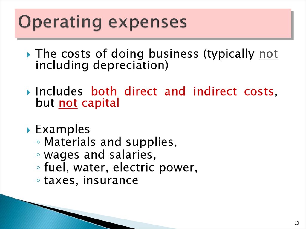
10. Operating expenses

The costs of doing business (typically not
including depreciation)
Includes both direct and indirect costs,
but not capital
Examples
◦ Materials and supplies,
◦ wages and salaries,
◦ fuel, water, electric power,
◦ taxes, insurance
10

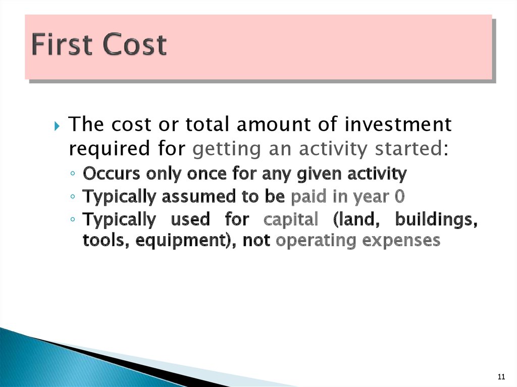
11. First Cost

The cost or total amount of investment
required for getting an activity started:
◦ Occurs only once for any given activity
◦ Typically assumed to be paid in year 0
◦ Typically used for capital (land, buildings,
tools, equipment), not operating expenses
11

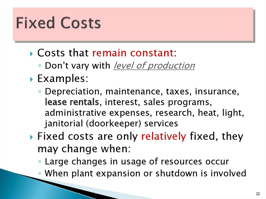
12. Fixed Costs

Costs that remain constant:
◦ Don’t vary with level of production
Examples:
◦ Depreciation, maintenance, taxes, insurance,
lease rentals, interest, sales programs,
administrative expenses, research, heat, light,
janitorial (doorkeeper) services
Fixed costs are only relatively fixed, they
may change when:
◦ Large changes in usage of resources occur
◦ When plant expansion or shutdown is involved
12

13. Variable Costs

Costs that vary with activity level:
◦ E.g., with number of units produced
◦ Typically only direct costs
◦ May (or may not) remain constant per
unit of product
Examples:
◦ Materials costs, direct labor, direct
electric power
13

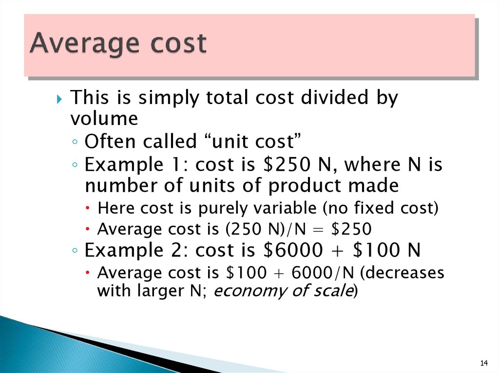
14. Average cost

This is simply total cost divided by
volume
◦ Often called “unit cost”
◦ Example 1: cost is $250 N, where N is
number of units of product made
Here cost is purely variable (no fixed cost)
Average cost is (250 N)/N = $250
◦ Example 2: cost is $6000 + $100 N
Average cost is $100 + 6000/N (decreases
with larger N; economy of scale)
14

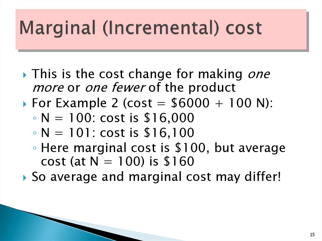
15. Marginal (Incremental) cost

This is the cost change for making one
more or one fewer of the product
For Example 2 (cost = $6000 + 100 N):
◦ N = 100: cost is $16,000
◦ N = 101: cost is $16,100
◦ Here marginal cost is $100, but average
cost (at N = 100) is $160
So average and marginal cost may differ!
15

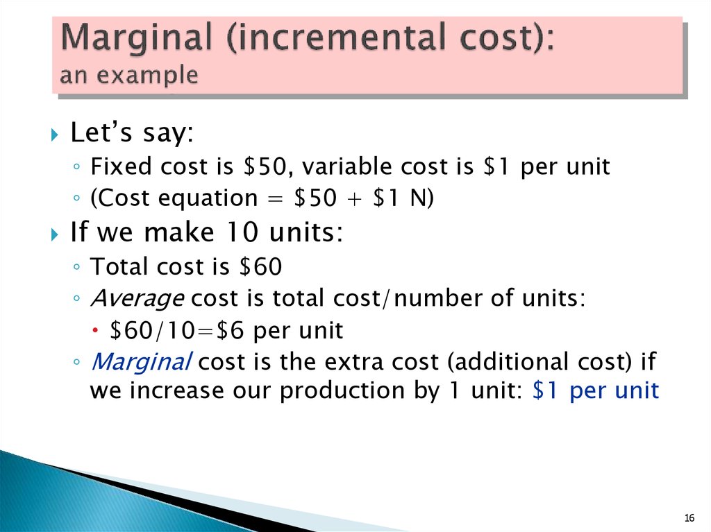
16. Marginal (incremental cost): an example

Let’s say:
◦ Fixed cost is $50, variable cost is $1 per unit
◦ (Cost equation = $50 + $1 N)
If we make 10 units:
◦ Total cost is $60
◦ Average cost is total cost/number of units:
$60/10=$6 per unit
◦ Marginal cost is the extra cost (additional cost) if
we increase our production by 1 unit: $1 per unit
16

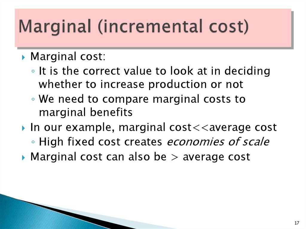
17. Marginal (incremental cost)

Marginal cost:
◦ It is the correct value to look at in deciding
whether to increase production or not
◦ We need to compare marginal costs to
marginal benefits
In our example, marginal cost<<average cost
◦ High fixed cost creates economies of scale
Marginal cost can also be > average cost
17

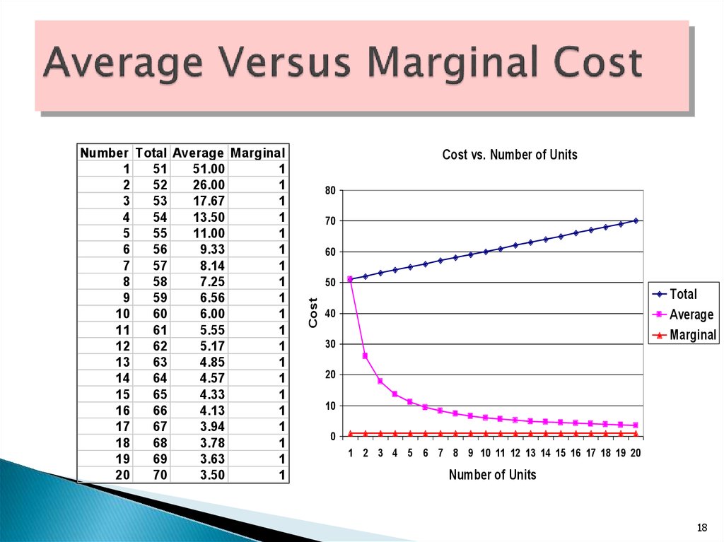
18. Average Versus Marginal Cost

Cost vs. Number of Units
80
70
60
50
Cost
Number Total Average Marginal
1
51
51.00
1
2
52
26.00
1
3
53
17.67
1
4
54
13.50
1
5
55
11.00
1
6
56
9.33
1
7
57
8.14
1
8
58
7.25
1
9
59
6.56
1
10
60
6.00
1
11
61
5.55
1
12
62
5.17
1
13
63
4.85
1
14
64
4.57
1
15
65
4.33
1
16
66
4.13
1
17
67
3.94
1
18
68
3.78
1
19
69
3.63
1
20
70
3.50
1
Total
Average
Marginal
40
30
20
10
0
1 2 3 4 5 6 7 8 9 10 11 12 13 14 15 16 17 18 19 20
Number of Units
18

19. Marginal (incremental cost)

Because
is the change in quantity
of labor that affects a one unit change
in output, this implies that this equals
1/MPL (marginal product of labor)
So, when marginal cost is increasing (decreasing) the
marginal product of labor is decreasing (increasing)
19

20. Recurring and Nonrecurring Costs

Recurring are the costs that are repetitive
All variable costs are recurring, but not all
recurring costs have to be variable
A fixed cost can be recurring cost, e.g. Office space
rental for architectural and engineering service
An example of a nonrecurring cost can be the cost
of constructing a plant or purchasing a piece of
land
20

21. Opportunity cost

is what you have to give up to
get something
◦ Often expressed in dollar terms; but not always:
Opportunity cost of this lecture is 1 hour’s sleep, or
more
21

22. Sunk Costs

Sunk costs are costs that can’t be
recovered
◦ Not the same as past costs
◦ Sunk costs are generally irrelevant to decision
Example:
◦ If a firm sinks $1 million on an enterprise
software installation, that cost is "sunk" because
it was a one-time thing and cannot be recovered
once expended.
◦ Room painting
22

23. Life-cycle cost

This is the total cost for a system, machine,
project, etc. during its service life
Major subdivisions:
◦ Acquisition cost
◦ Operation cost
◦ Maintenance cost
23

24. Cost-Estimating Methods

Accounting Method
Engineering Method
Statistical Method
24

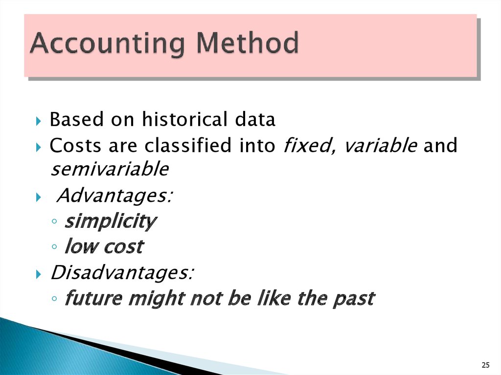
25. Accounting Method

Based on historical data
Costs are classified into fixed, variable and
semivariable
Advantages:
◦ simplicity
◦ low cost
Disadvantages:
◦ future might not be like the past
25

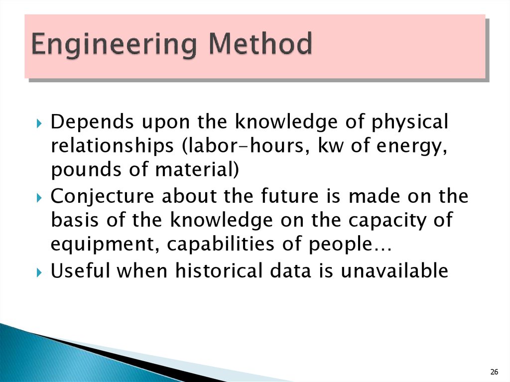
26. Engineering Method

Depends upon the knowledge of physical
relationships (labor-hours, kw of energy,
pounds of material)
Conjecture about the future is made on the
basis of the knowledge on the capacity of
equipment, capabilities of people…
Useful when historical data is unavailable
26

27. Statistical Method

Uses statistical tools (from simple graphs to
complex regressions)
Objective is to find a functional relationship
between changes in costs and factors like
output rate
The most reliable method when data is
available
27

28.

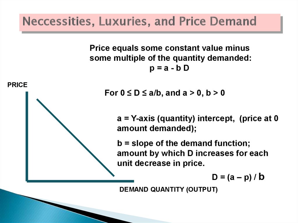
Neccessities, Luxuries, and Price Demand
Price equals some constant value minus
some multiple of the quantity demanded:
p=a-bD
PRICE
For 0 ≤ D ≤ a/b, and a > 0, b > 0
a = Y-axis (quantity) intercept, (price at 0
amount demanded);
b = slope of the demand function;
amount by which D increases for each
unit decrease in price.
D = (a – p) / b
DEMAND QUANTITY (OUTPUT)

29.

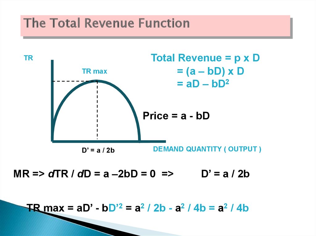
The Total Revenue Function
TR
TR max
Total Revenue = p x D
= (a – bD) x D
= aD – bD2
Price = a - bD
D’ = a / 2b
DEMAND QUANTITY ( OUTPUT )
MR => dTR / dD = a –2bD = 0 =>
D’ = a / 2b
TR max = aD’ - bD’2 = a2 / 2b - a2 / 4b = a2 / 4b

30. Cost, Volume, and Breakeven point Relationship

Profit = (aD - bD2) – (CF + CvD) = - bD2 + (a-Cv)D-CF
Max Profit => d(profit)/dD = 0 =>
a – Cv - 2bD = 0
D* = a – Cv / - 2b
30

31. Cost, Volume, and Breakeven point Relationship

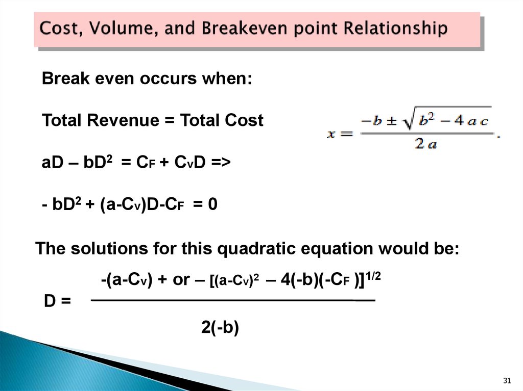
Break even occurs when:
Total Revenue = Total Cost
aD – bD2 = CF + CvD =>
- bD2 + (a-Cv)D-CF = 0
The solutions for this quadratic equation would be:
-(a-Cv) + or – [(a-Cv)2 – 4(-b)(-CF )]1/2
D=
2(-b)
31

32.

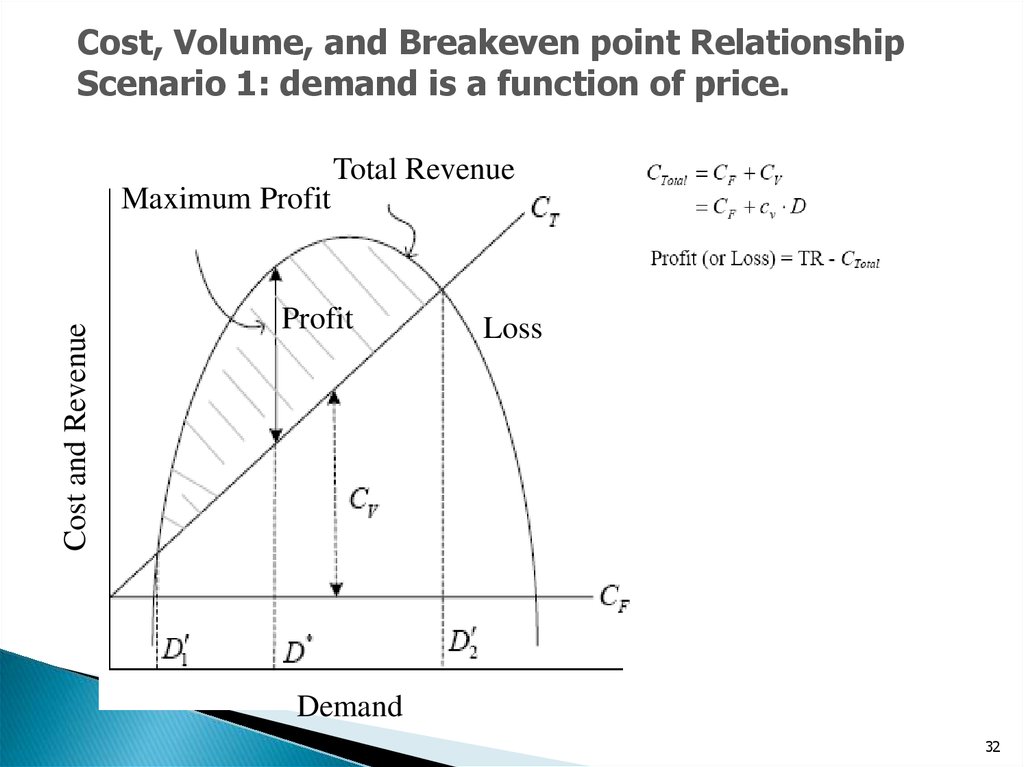
Cost, Volume, and Breakeven point Relationship
Scenario 1: demand is a function of price.
Total Revenue
Cost and Revenue
Maximum Profit
Profit
Loss
Demand
32

33.

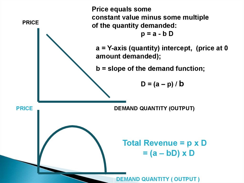
PRICE
Price equals some
constant value minus some multiple
of the quantity demanded:
p=a-bD
a = Y-axis (quantity) intercept, (price at 0
amount demanded);
b = slope of the demand function;
D = (a – p) / b
PRICE
DEMAND QUANTITY (OUTPUT)
Total Revenue = p x D
= (a – bD) x D
DEMAND QUANTITY ( OUTPUT )

34.

Maximum
Profit
Cost / Revenue
Marginal
( Incremental) Cost
Profit is maximum where
Total Revenue exceeds
Total Cost by greatest amount
Marginal
Revenue
Quantity ( Output )
Demand
Cost / Revenue
Ct
Profit
Total Revenue
Cf
D’1
D*
D’2
D’1 and D’2 are breakeven points
Quantity ( Output )
Demand

35. Example 2.6

A Company produces an electronic timing switch
that is used in consumer and commercial products
made by several other manufacturing firms. The
fixed cost (CF) is $73,000 per month, and the variable
cost (cv) is $83 per unit. The selling price per unit is
p = $180 – 0.02(D)
a) Determine the optimal volume for this product, and
b) Find the volumes at which breakeven occurs; that
is, what is the domain of profitable demand?
35

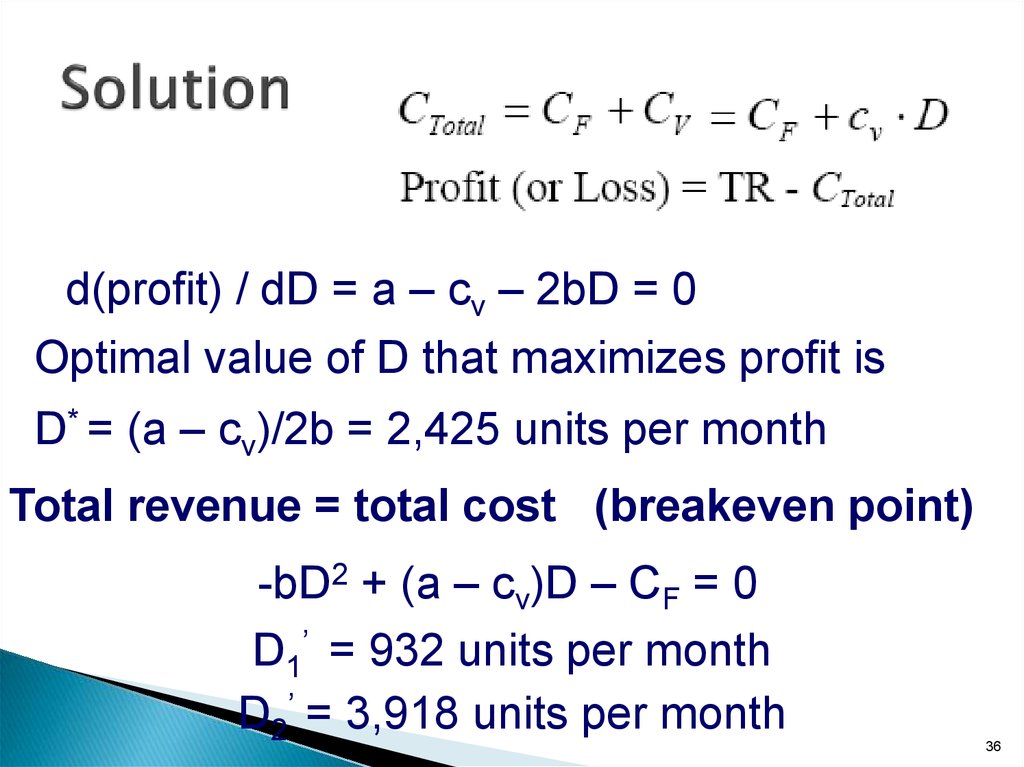
36. Solution

d(profit) / dD = a – cv – 2bD = 0
Optimal value of D that maximizes profit is
D* = (a – cv)/2b = 2,425 units per month
Total revenue = total cost (breakeven point)
-bD2 + (a – cv)D – CF = 0
D1’ = 932 units per month
D2’ = 3,918 units per month
36

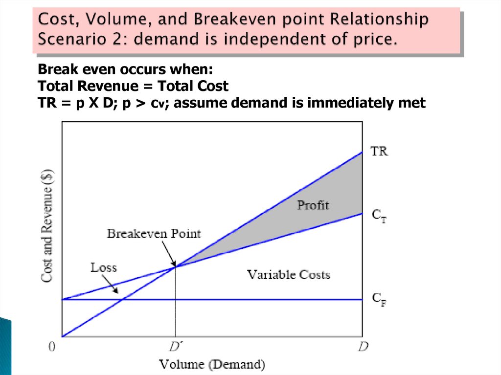
37. Cost, Volume, and Breakeven point Relationship Scenario 2: demand is independent of price.

Break even occurs when:
Total Revenue = Total Cost
TR = p X D; p > cv; assume demand is immediately met

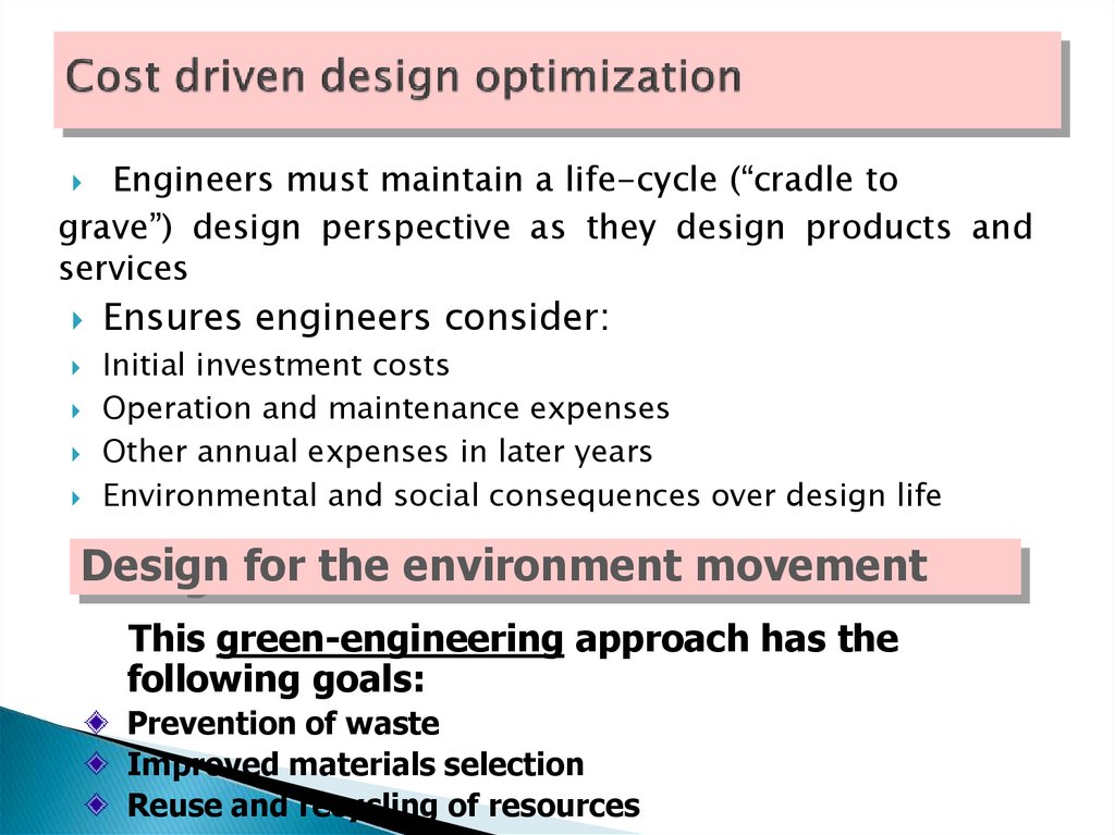
38. Cost driven design optimization

Engineers must maintain a life-cycle (“cradle to
grave”) design perspective as they design products and
services
Ensures engineers consider:
Initial investment costs
Operation and maintenance expenses
Other annual expenses in later years
Environmental and social consequences over design life
Design for the environment movement
This green-engineering approach has the
following goals:
Prevention of waste
Improved materials selection
Reuse and recycling of resources

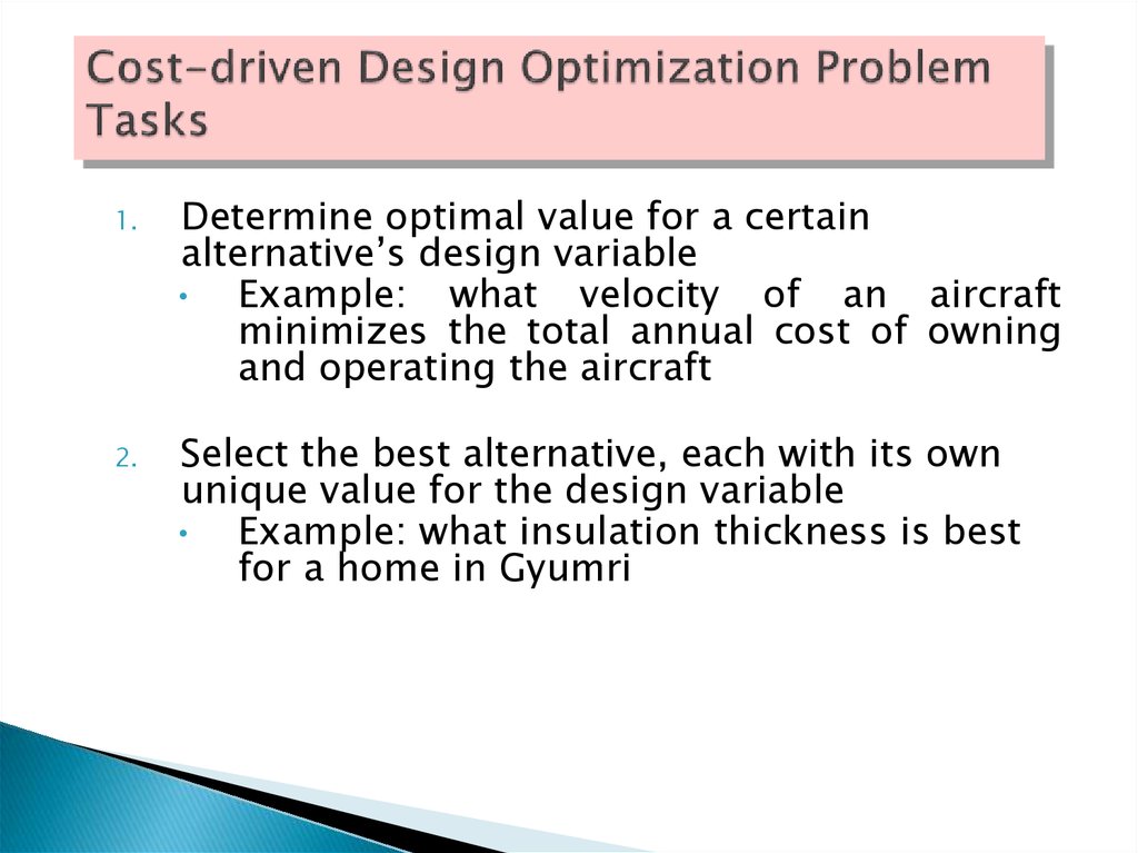
39. Cost-driven Design Optimization Problem Tasks

1.
2.
Determine optimal value for a certain
alternative’s design variable
• Example: what velocity of an aircraft
minimizes the total annual cost of owning
and operating the aircraft
Select the best alternative, each with its own
unique value for the design variable
• Example: what insulation thickness is best
for a home in Gyumri

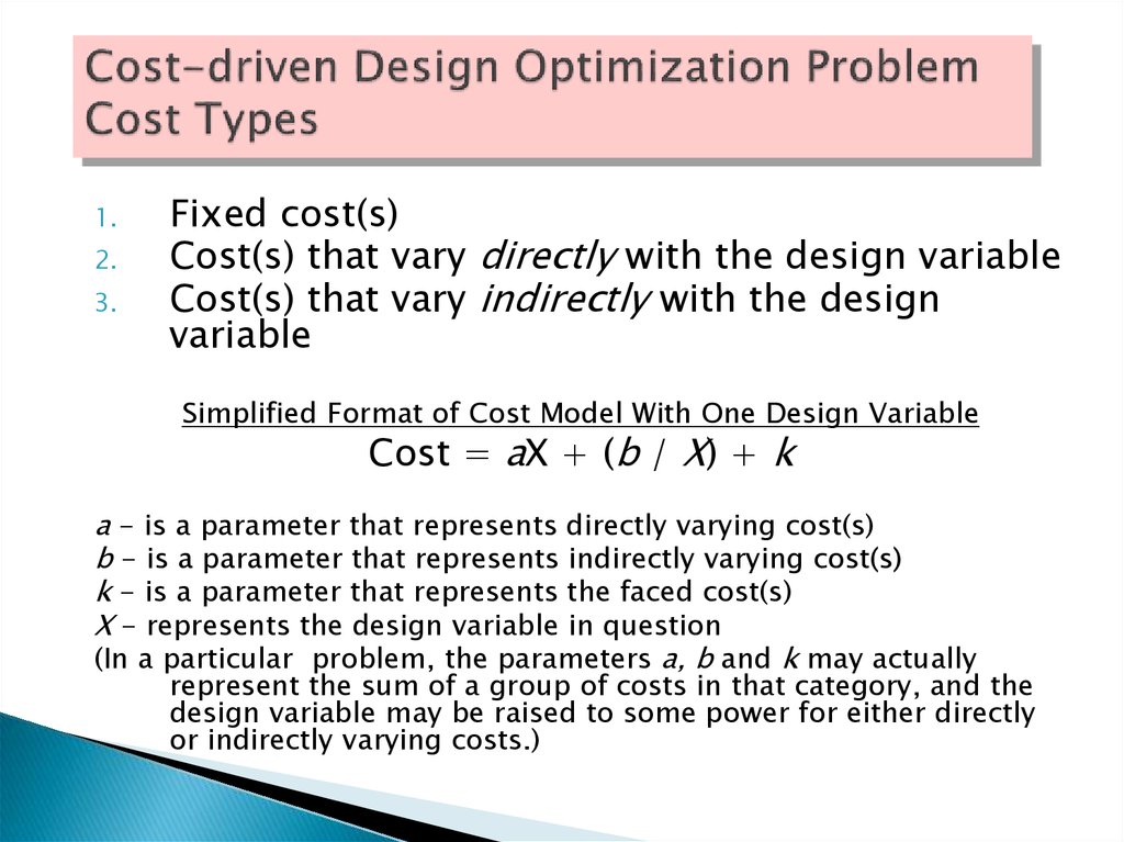
40. Cost-driven Design Optimization Problem Cost Types

1.
2.
3.
Fixed cost(s)
Cost(s) that vary directly with the design variable
Cost(s) that vary indirectly with the design
variable
Simplified Format of Cost Model With One Design Variable
Cost = aX + (b / X) + k
a - is a parameter that represents directly varying cost(s)
b - is a parameter that represents indirectly varying cost(s)
k - is a parameter that represents the faced cost(s)
X - represents the design variable in question
(In a particular problem, the parameters a, b and k may actually
represent the sum of a group of costs in that category, and the
design variable may be raised to some power for either directly
or indirectly varying costs.)

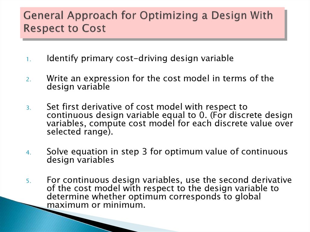
41. General Approach for Optimizing a Design With Respect to Cost

1.
Identify primary cost-driving design variable
2.
Write an expression for the cost model in terms of the
design variable
3.
4.
5.
Set first derivative of cost model with respect to
continuous design variable equal to 0. (For discrete design
variables, compute cost model for each discrete value over
selected range).
Solve equation in step 3 for optimum value of continuous
design variables
For continuous design variables, use the second derivative
of the cost model with respect to the design variable to
determine whether optimum corresponds to global
maximum or minimum.

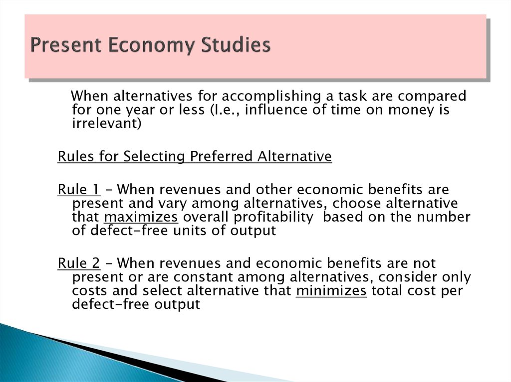
42. Present Economy Studies

When alternatives for accomplishing a task are compared
for one year or less (I.e., influence of time on money is
irrelevant)
Rules for Selecting Preferred Alternative
Rule 1 – When revenues and other economic benefits are
present and vary among alternatives, choose alternative
that maximizes overall profitability based on the number
of defect-free units of output
Rule 2 – When revenues and economic benefits are not
present or are constant among alternatives, consider only
costs and select alternative that minimizes total cost per
defect-free output

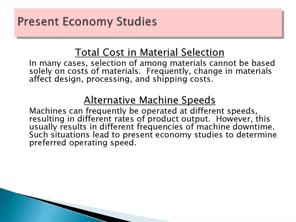
43. Present Economy Studies

Total Cost in Material Selection
In many cases, selection of among materials cannot be based
solely on costs of materials. Frequently, change in materials
affect design, processing, and shipping costs.
Alternative Machine Speeds
Machines can frequently be operated at different speeds,
resulting in different rates of product output. However, this
usually results in different frequencies of machine downtime.
Such situations lead to present economy studies to determine
preferred operating speed.

44. Present Economy Studies

Make Versus Purchase (Outsourcing) Studies
A company may choose to produce an item in house, rather than
purchase from a supplier at a price lower than production costs
if:
direct, indirect or overhead costs are incurred regardless of whether
the item is purchased from an outside supplier, and
• The incremental cost of producing the item in the short run is less
than the supplier’s price.
The relevant short-run costs of the make versus purchase
decisions are the incremental costs incurred and the opportunity
costs of resources

45. Present Economy Studies

Make Versus Purchase (Outsourcing) Studies
Opportunity costs may become significant when
in-house manufacture of an item causes other
production opportunities to be foregone (E.G.,
insufficient capacity)
In the long run, capital investments in additional
manufacturing plant and capacity are often feasible
alternatives to outsourcing.