Similar presentations:
Acoustic Waveform Processing
1. Acoustic Waveform Processing
Workflow primerWorking together
for a safer world
2. System requirements
x64 better because wells can be ~4GB
Memory: overhead is about 250MB per core
CPU: more physical cores = faster, currently
tops out at using 8 physical cores (Intel’s
Hyperthreading doesn’t count as extra cores)
Matlab 2015a: you’re prompted to install it if it is
not there.
Patience because processing is time
consuming
3. Introducing the data
This module processes sound waves:
examining the ‘types’ of waves their speed
through the rock
The speed of sound in rock can tell us about
the type of rock, fluid content and what stresses
the rock is under
A typical Acoustic tool is pictured
Some standard-looking raw-data is show
bottom
4. Designed-for Workflows
Most often, our clients are looking to verify the
work of others with this module (so our results
should generally agree)
We see a few different uses of the module:
1.
Re-working other’s processed data to
correct their errors
2.
Re-processing the raw data to verify
someone else’s interpretation
3.
Re-processing the raw data to derive new
information
Very often the outputs of this module are inputs
to other modules (from PhiSw to Geomechanics)
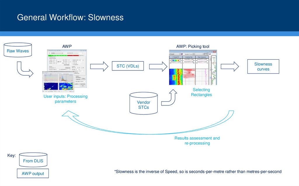
5. General Workflow: Slowness
AWPAWP: Picking tool
Raw Waves
Slowness
curves
STC (VDLs)
User inputs: Processing
parameters
Selecting
Rectangles
Vendor
STCs
Results assessment and
re-processing
Key:
From DLIS
AWP output
*Slowness is the inverse of Speed, so is seconds-per-metre rather than metres-per-second
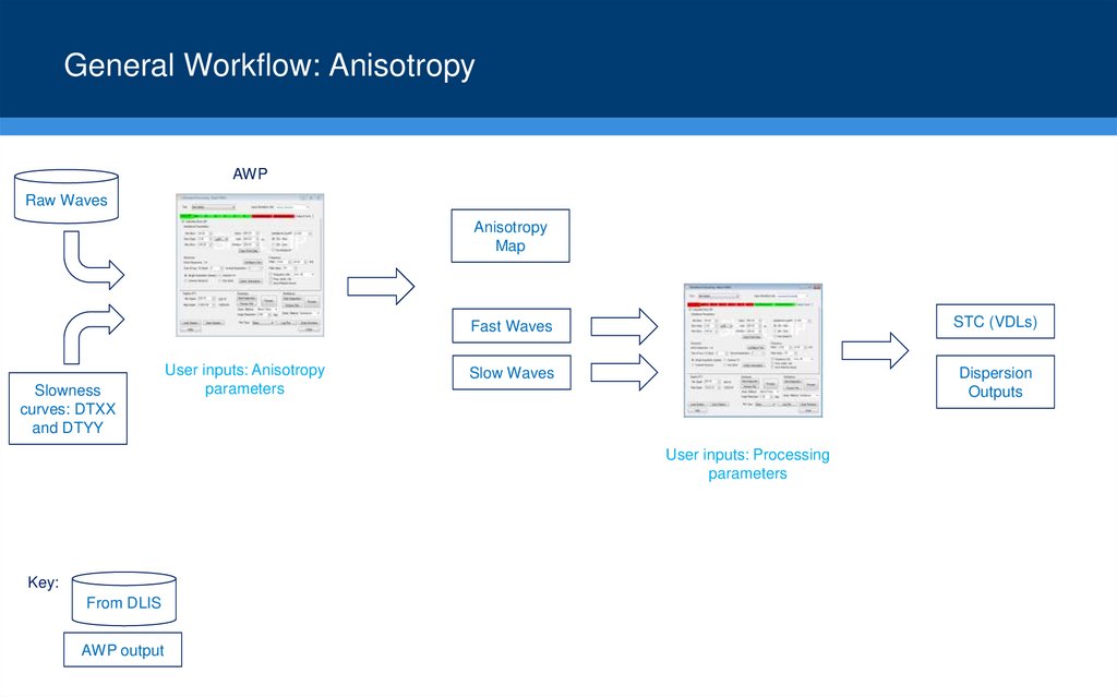
6. General Workflow: Anisotropy
AWPRaw Waves
Anisotropy
Map
Slowness
curves: DTXX
and DTYY
User inputs: Anisotropy
parameters
Fast Waves
STC (VDLs)
Slow Waves
Dispersion
Outputs
User inputs: Processing
parameters
Key:
From DLIS
AWP output
7. Workflow 1: Re-picking
AWPAWP: Picking tool
Raw Waves
Slowness
curves
STC (VDLs)
User inputs: Processing
parameters
Selecting
Rectangles
Vendor
STCs
Data Assessment and
personal interpretations
Slowness from other people’s processing
WORKFLOW 1: RE-PICKING
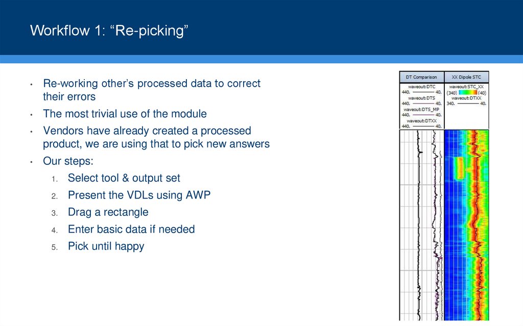
8. Workflow 1: “Re-picking”
Re-working other’s processed data to correct
their errors
The most trivial use of the module
Vendors have already created a processed
product, we are using that to pick new answers
Our steps:
1.
Select tool & output set
2.
Present the VDLs using AWP
3.
Drag a rectangle
4.
Enter basic data if needed
5.
Pick until happy
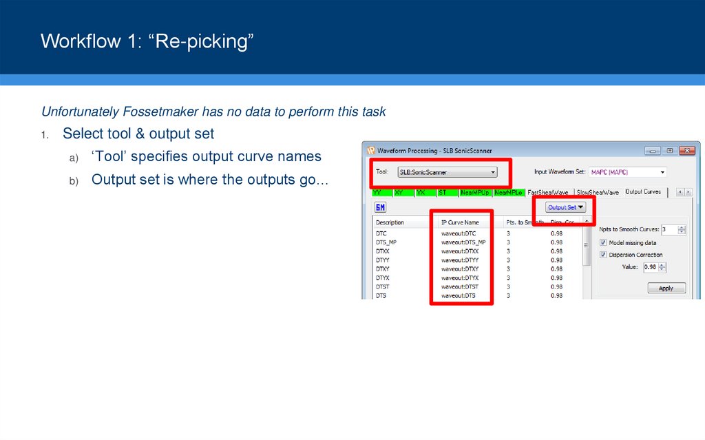
9. Workflow 1: “Re-picking”
Unfortunately Fossetmaker has no data to perform this task1.
Select tool & output set
a)
‘Tool’ specifies output curve names
b)
Output set is where the outputs go…
10. Workflow 1: “Re-picking”
Unfortunately Fossetmaker has no data to perform this task1.
2.
Select tool & output set
a)
‘Tool’ specifies output curve names
b)
Output set is where the outputs go…
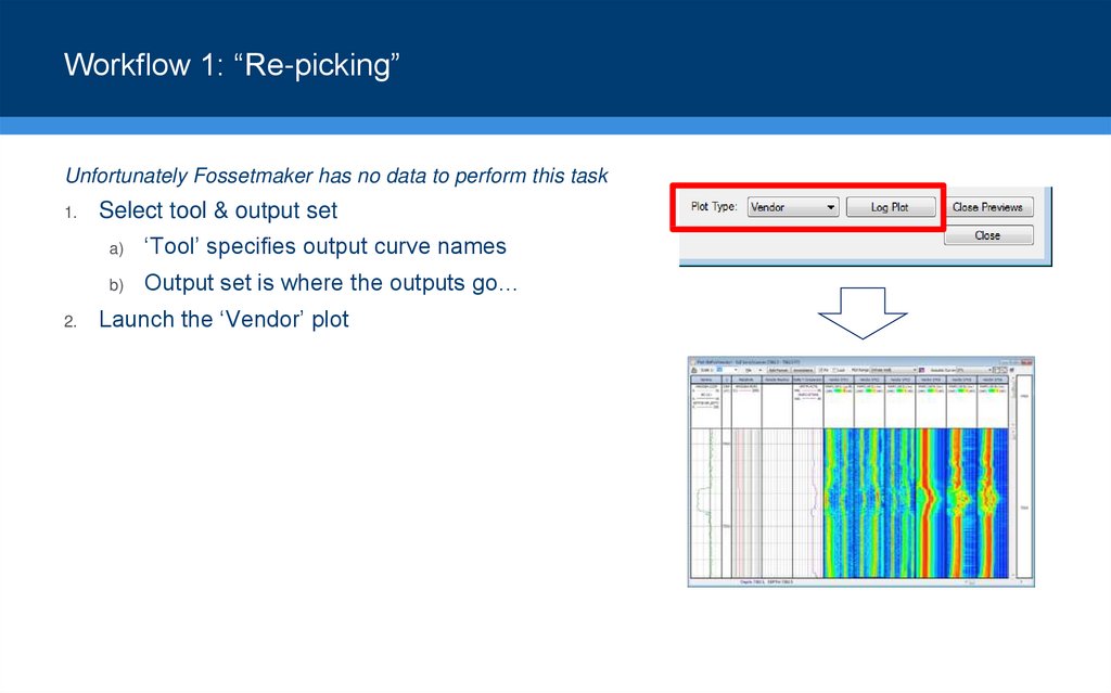
Launch the ‘Vendor’ plot
11. Workflow 1: “Re-picking”
Unfortunately Fossetmaker has no data to perform this task1.
Select tool & output set
a)
‘Tool’ specifies output curve names
b)
Output set is where the outputs go…
2.
Launch the ‘Vendor’ plot
3.
Hit the Drop-down for the curve you want to make
12. Workflow 1: “Re-picking”
Unfortunately Fossetmaker has no data to perform this task1.
Select tool & output set
a)
‘Tool’ specifies output curve names
b)
Output set is where the outputs go…
2.
Launch the ‘Vendor’ plot
3.
Hit the Drop-down for the curve you want to make
4.
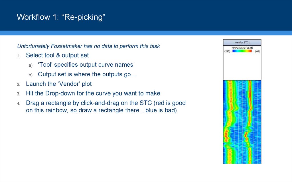
Drag a rectangle by click-and-drag on the STC (red is good
on this rainbow, so draw a rectangle there…blue is bad)
13. Workflow 1: “Re-picking”
Unfortunately Fossetmaker has no data to perform this task1.
Select tool & output set
a)
‘Tool’ specifies output curve names
b)
Output set is where the outputs go…
2.
Launch the ‘Vendor’ plot
3.
Hit the Drop-down for the curve you want to make
4.
Drag a rectangle by click-and-drag on the STC (red is good
on this rainbow, so draw a rectangle there…blue is bad)
5.
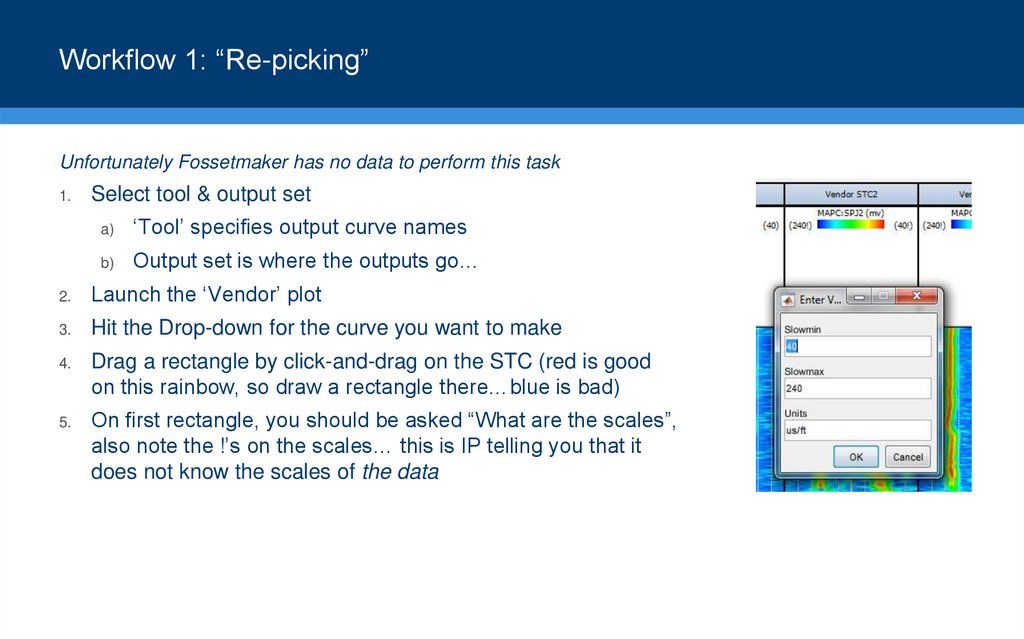
On first rectangle, you should be asked “What are the scales”,
also note the !’s on the scales… this is IP telling you that it
does not know the scales of the data
14. Workflow 1: “Re-picking”
Unfortunately Fossetmaker has no data to perform this task1.
Select tool & output set
a)
‘Tool’ specifies output curve names
b)
Output set is where the outputs go…
2.
Launch the ‘Vendor’ plot
3.
Hit the Drop-down for the curve you want to make
4.
Drag a rectangle by click-and-drag on the STC (red is good
on this rainbow, so draw a rectangle there…blue is bad)
5.
6.
On first rectangle, you should be asked “What are the scales”,
also note the !’s on the scales… this is IP telling you that it
does not know the scales of the data
Rectangle picking can continue, picking whatever…
15. Workflow 1: “Re-picking”
Notes on Rectangle picking:Selections are made from one VDL at a time
Default scales are 0..1 some vendors use 0..100!
3 curves are made: the curve name you picked from the
dropdown (step 3 above), a smoothed version and a _psv
“peak semblance value” curve, representing the height of the
VDL colour map and is a quality indicator
16. Workflow 2: Processing Raw
AWPAWP: Picking tool
Raw Waves
Slowness
curves
STC (VDLs)
User inputs: Processing
parameters
Selecting
Rectangles
Vendor
STCs
Data Assessment and
personal interpretations
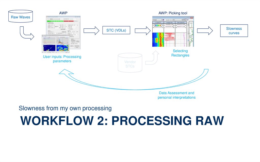
Slowness from my own processing
WORKFLOW 2: PROCESSING RAW
17. Workflow 2: Processing Raw Waves
The picking part of this workflow is the same
Bulk of the processing work here
Our steps:
1.
2.
Select tool, input & output sets
Deactivate the modes you don’t want to
process now
3.
View Diagnostic pane
4.
Set up parameters in Diag. or manual
5.
Process or Preview
6.
Return to step 4, refining parameters or
processing interval
18. Workflow 2: Processing Raw Waves
1.Select tool, input & output set
a)
‘Tool’ specifies the ‘modes’ (Short_MP, MP, ST
etc..) and output curve names
b)
Output set in Output Curve tabs is where some
outputs go
c)
Output set in Configure Tool is where most
Array outputs go
d)
Input Waveform Set is where to pick up the raw
waves from (shown in Configure Tool)
You should inspect both Output Curves
19. Workflow 2: Processing Raw Waves
2.Pick the Modes you want:
a)
b)
Un-check the “Calculate ??” to turn off ??
Today we want to process MP but not any
others
Grey tab = no process
Red tab = no waves, can’t process
Green tab = have waves will process
20. Workflow 2: Processing Raw Waves
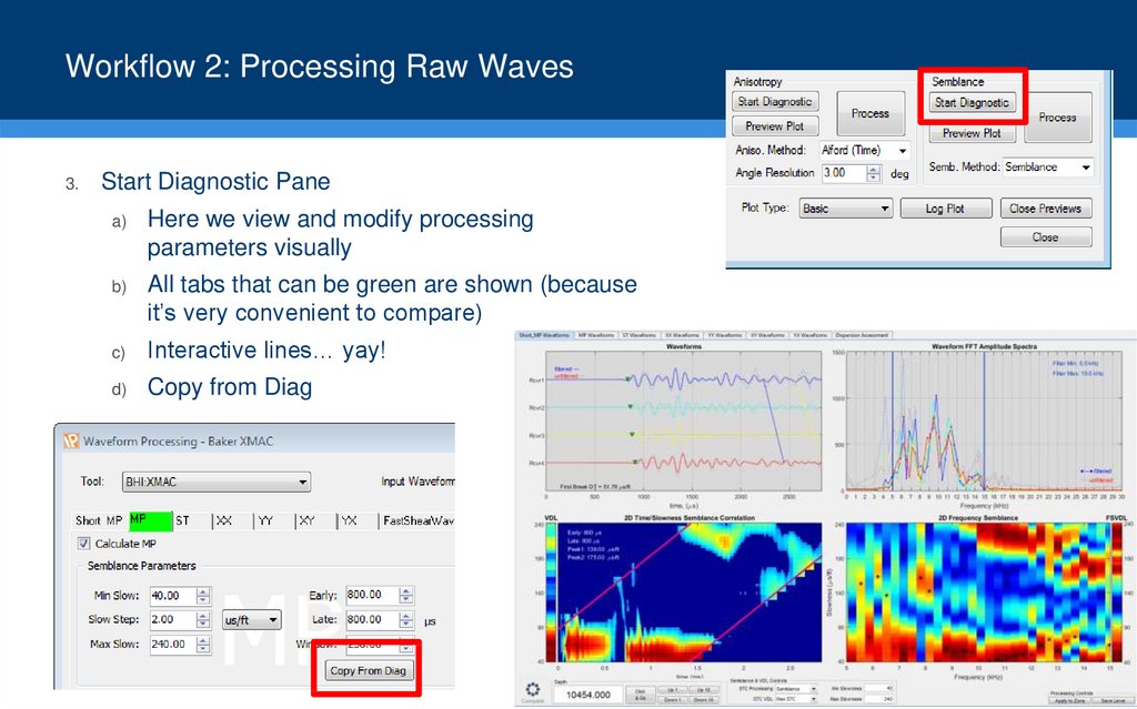
3.Start Diagnostic Pane
a)
Here we view and modify processing
parameters visually
b)
All tabs that can be green are shown (because
it’s very convenient to compare)
c)
Interactive lines… yay!
d)
Copy from Diag
21. Workflow 2: Processing Raw Waves
3.Process whole well
a)
Using Diagnostic we’d pick general parameters
that work most places and process the whole
well
b)
Hit the Process button
c)
Processing can take a while (about a minute for
MP on this well)
d)
Output is an STC_MP, which we can use in the
picking process outlined in Workflow 1
e)
Launch a ‘Basic’ Log plot, then pick DTC etc.
like in Workflow 1
22. Workflow 2: Processing Raw Waves
4.Process whole well
a)
After seeing the whole well, we may choose to
reprocess all or part-sections
b)
Ordinarily this is driven by inspecting problem
sections with Diagnostic window, re-adjusting
parameters and processing the bad parts again
c)
Once happy with the STC outcome, can re-pick
DTC etc. again
23. Workflow 2: Processing Raw Waves
Notes on processing:Like everything else in IP, there’s no ‘right’ answer
Changing parameters can make yours look very
different: don’t get too hung up
There are many different ways to process and
interpret (NthRoot, Common Rx, VDL Max/Sum and
lots of parameters…) so expect variation
But! Same settings should make the same answer
in the same well
24. Workflow 3: Anisotropy
AWPRaw Waves
Anisotropy
Map
Slowness
curves: DTXX
and DTYY
User inputs: Anisotropy
parameters
Fast Waves
STC (VDLs)
Slow Waves
Dispersion
Outputs
User inputs: Processing
parameters
Azimuthally changing slowess
WORKFLOW 3: ANISOTROPY
25. Workflow 3: Anisotropy Processing
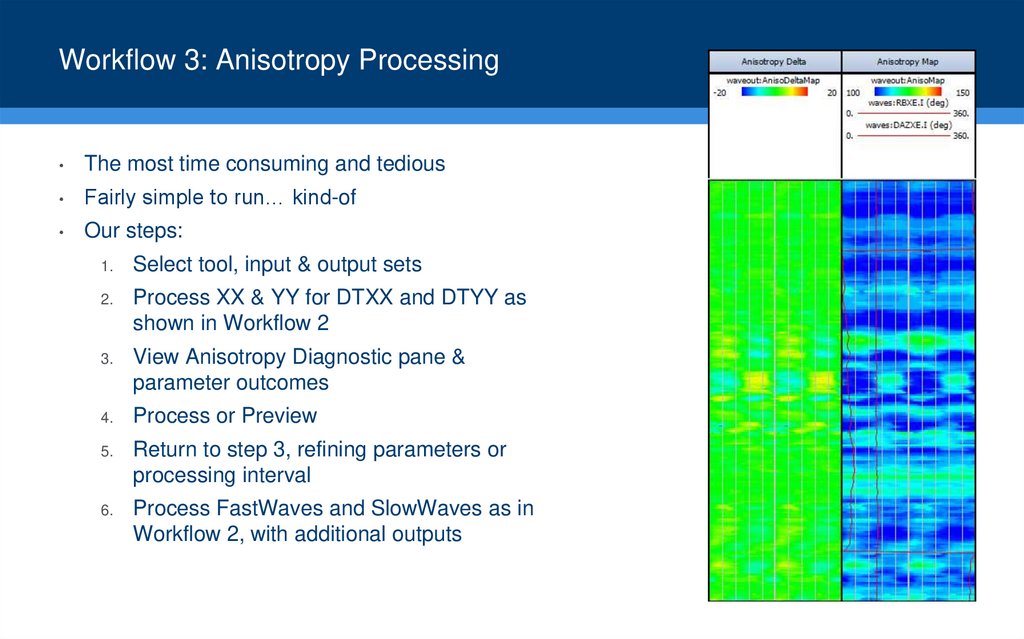
The most time consuming and tedious
Fairly simple to run… kind-of
Our steps:
1.
Select tool, input & output sets
2.
Process XX & YY for DTXX and DTYY as
shown in Workflow 2
3.
View Anisotropy Diagnostic pane &
parameter outcomes
4.
Process or Preview
5.
Return to step 3, refining parameters or
processing interval
6.
Process FastWaves and SlowWaves as in
Workflow 2, with additional outputs
26. Workflow 3: Anisotropy Processing
1.Select tool, input & output set
a)
‘Tool’ specifies the ‘modes’ (Short_MP, MP, ST
etc..) and output curve names
b)
Output set in Output Curve tabs is where some
outputs go
c)
Output set in Configure Tool is where most
Array outputs go
d)
Input Waveform Set is where to pick up the raw
waves from (shown in Configure Tool)
You should inspect both Output Curves
27. Workflow 3: Anisotropy Processing
2.Process XX & YY for DTXX and DTYY
a)
Using Workflow 2 you need to create a DTXX
and DTYY; invalid DTXX or invalid DTYY
prevent anisotropy being calculated at that
depth
28. Workflow 3: Anisotropy Processing
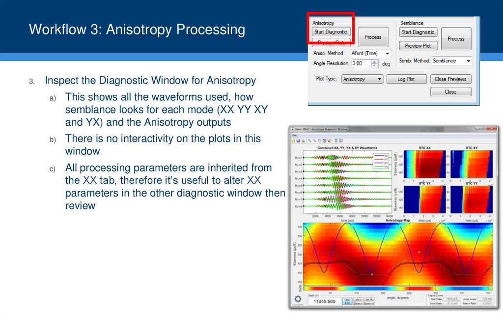
3.Inspect the Diagnostic Window for Anisotropy
a)
This shows all the waveforms used, how
semblance looks for each mode (XX YY XY
and YX) and the Anisotropy outputs
b)
There is no interactivity on the plots in this
window
c)
All processing parameters are inherited from
the XX tab, therefore it’s useful to alter XX
parameters in the other diagnostic window then
review
29. Workflow 3: Anisotropy Processing
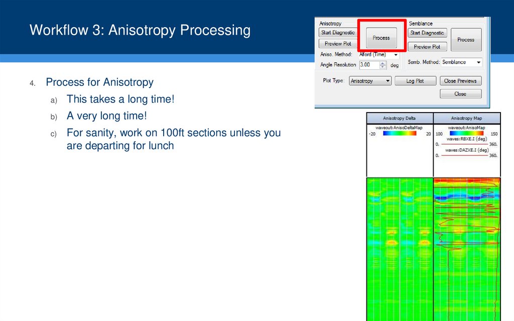
4.Process for Anisotropy
a)
This takes a long time!
b)
A very long time!
c)
For sanity, work on 100ft sections unless you
are departing for lunch
30. Workflow 3: Anisotropy Processing
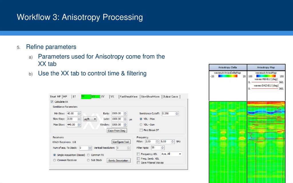
5.Refine parameters
a)
Parameters used for Anisotropy come from the
XX tab
b)
Use the XX tab to control time & filtering
31. Workflow 3: Anisotropy Processing
6.Process FastWaves and SlowWaves
a)
Switch the Input Waveform Set to pick up
FastShearWaves & SlowShearWaves
b)
Process these waves like Workflow 2, but with
‘Frequency VDL’ and ‘Freq. Semb. VDL’
checked
c)
Comparison of FVDL2’s can be made
32.
First name Last namePosition
Unit/ Department
T +44 (0)23 2345 5432 E [email protected]
Lloyd’s Register [Entity]
71 Fenchurch Street, London EC3M 4BS
Working together
for a safer world
Lloyd’s Register and variants of it are trading names of Lloyd’s Register Group Limited, its subsidiaries and affiliates.
Copyright © Lloyd’s Register [Entity]. 2013. A member of the Lloyd’s Register group.














 english


