Heuristics for the TSP

1. ACO, Lecture 10, Heuristics for the TSP

Boris Goldengorin
ACO Spring 2024
1

2. Motivation

• Heuristics clearly are necessary for NP-complete (hard)
problems if we expect to solve them in reasonable
amounts of computer time. Heuristics also are useful in
speeding up the convergence of exact optimization
algorithms, typically by providing good starting solutions.
Heuristics can be classified into several categories.
ACO Spring 2024
2

3. Construction and Improvement

• Construction heuristics build a feasible solution one
component at a time. In graph applications, for example,
one might add edges to a solution one at a time until a
certain structure such as a tree is realized. Such
heuristics are often used to generate initial feasible
solutions to a problem.
• Improvement heuristics start with a complete feasible
solution to a problem and successively improve it
through a sequence of exchanges or mergers. For
instance, one might with begin a cycle that represents a
feasible solution to the TSP and try to remove some
edges that can be replaced by others at a lower cost
while still maintaining feasibility.
ACO Spring 2024
3

4. Partitioning and Decomposition, and Specialized Methods

• Partitioning and decomposition refer to methods that break a
problem down into smaller components that can be solved in
sequence or independently. We shall see one example of a heuristic
for the TSP that first finds a spanning tree in the graph and then
solves an auxiliary problem to construct a feasible solution. Another
example would be the partitioning of a planar graph into geographic
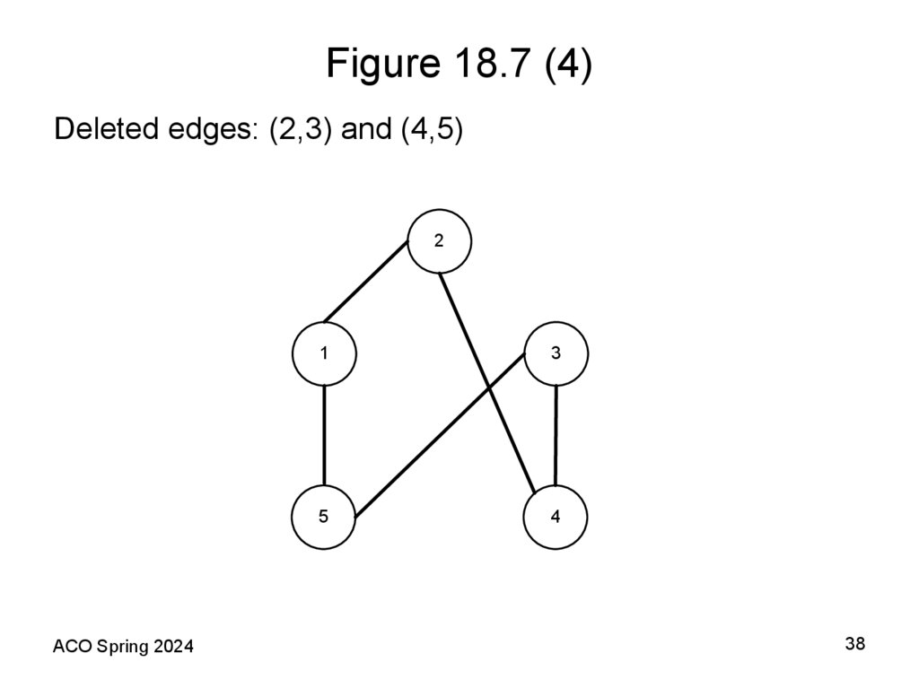
regions, solving a subproblem within each region, and merging the
solution into one overall solution.
• Many other special methods exist for certain problems that depend,
for example, on solving a relaxation of an ”integer” (cyclic or some
other discrete property of feasible solution) program, or applying
probabilistic analysis. These usually are problem dependent and
take advantage of special structures inherent in the problem.
ACO Spring 2024
4

5. Desirable characteristics of heuristic include

• 1. They run in a reasonable (polynomial) computational
time.
• 2. Solutions generally (as a rule) are close to optimal.
• 3. The probability of any one solution being very far from
optimal is small.
• 4. Storage requirements are small.
ACO Spring 2024
5

6.

Quality and Complexity
• The computational complexity of heuristics often can be
determined in the same manner as for exact algorithms.
In addition, we can sometimes compute worst-case
bounds on the deviation of the solution from optimality.
That is, we might be able to show that the heuristic
solution will be no more that some fixed percentage from
the optimal solution for any problem instance.
ACO Spring 2024
6

7. Worst-Case Analysis

• Since most complicated logistics problems, for example,
the Simple Plant Location Problem and Traveling
Salesman Problems, are NP-hard it is unlikely that
polynomial time algorithms will be developed for their
optimal solutions. Consequently, a great deal of work
has been devoted to the development and analyses of
heuristics. In this lecture we demonstrate one important
tool, referred as worst-case performance analysis, which
establishes the maximum deviation from optimality that
can occur for a given heuristic algorithm. We will
characterize the worst-case performance of a variety of
algorithms for the TSP.
ACO Spring 2024
7

8. Worst-Case Analysis (continued)

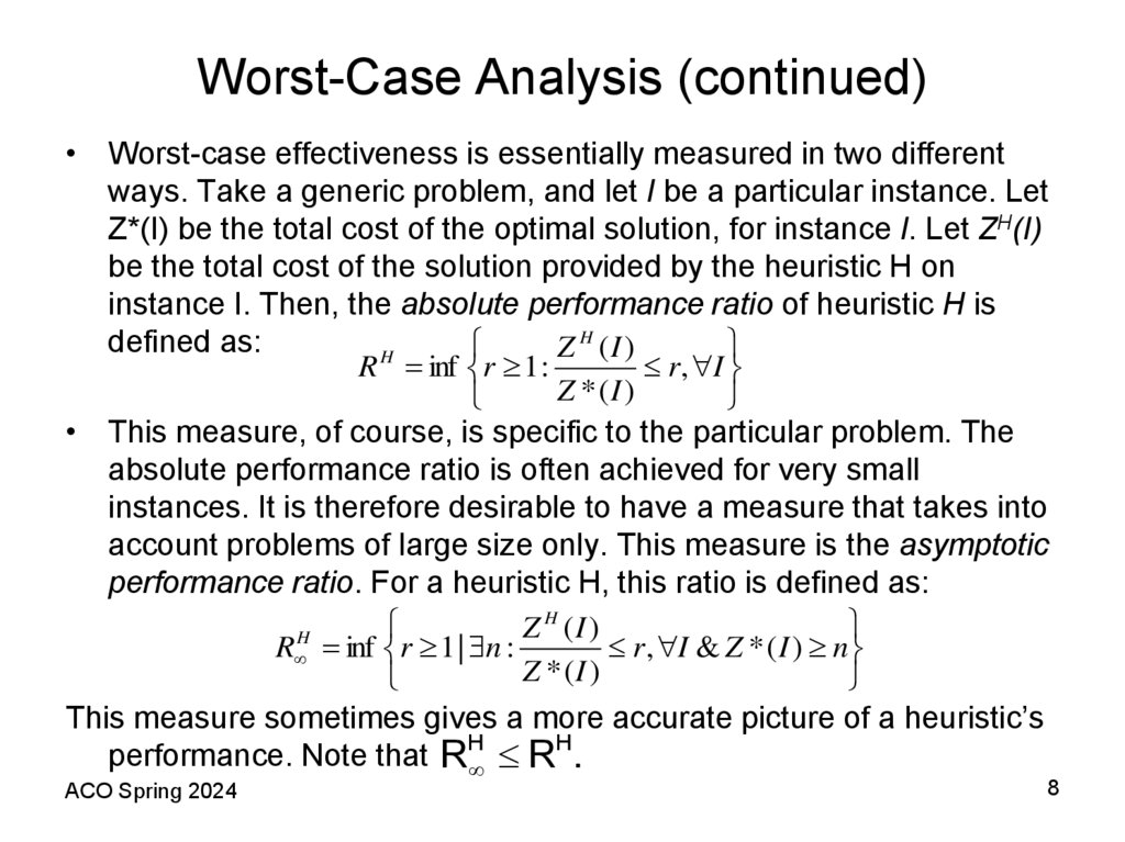
• Worst-case effectiveness is essentially measured in two different
ways. Take a generic problem, and let I be a particular instance. Let
Z*(I) be the total cost of the optimal solution, for instance I. Let ZH(I)
be the total cost of the solution provided by the heuristic H on
instance I. Then, the absolute performance ratio of heuristic H is
defined as:
Z H (I )
H
R inf r 1 :
r , I
Z * (I )
• This measure, of course, is specific to the particular problem. The
absolute performance ratio is often achieved for very small
instances. It is therefore desirable to have a measure that takes into
account problems of large size only. This measure is the asymptotic
performance ratio. For a heuristic H, this ratio is defined as:
Z H (I )
H
R inf r 1 | n :
r , I & Z * ( I ) n
Z
*
(
I
)
This measure sometimes gives a more accurate picture of a heuristic’s
H
H
performance. Note that R R .
ACO Spring 2024
8

9. Worst-Case Analysis – Theorem 1

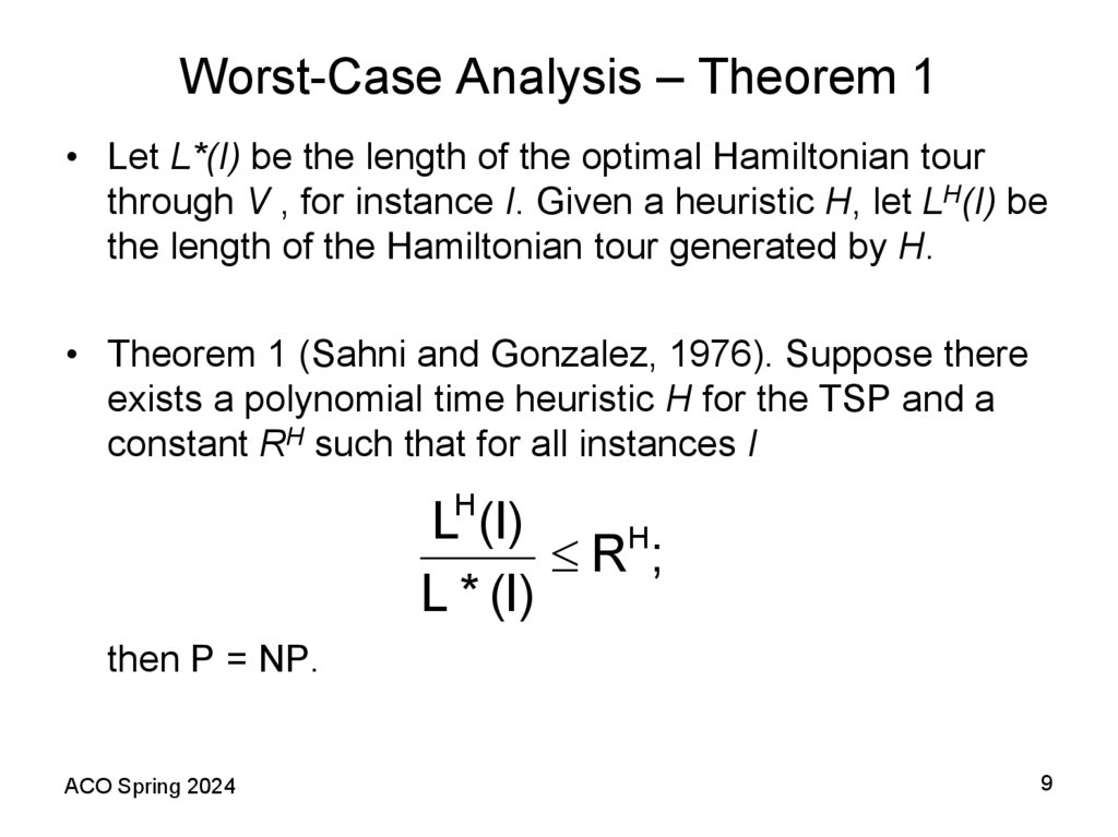
• Let L*(I) be the length of the optimal Hamiltonian tour
through V , for instance I. Given a heuristic H, let LH(I) be
the length of the Hamiltonian tour generated by H.
• Theorem 1 (Sahni and Gonzalez, 1976). Suppose there
exists a polynomial time heuristic H for the TSP and a
constant RH such that for all instances I
LH (I)
RH ;
L * (I)
then P = NP.
ACO Spring 2024
9

10. Worst-Case Analysis – Theorem 1 continued

• Theorem 1 implies that it is very unlikely that a
polynomial time heuristic for the TSP with a constant
absolute worst-case bound exists. However there is an
NP-hard version of the TSP that excludes the above
negative result. This is when the distance matrix c(i, j)
satisfies the following triangle inequality assumption:
i, j, k V c(i, j) c(i, k ) c(k, j)
• In many logistics environments, the triangle inequality
assumption is not a very restrictive one. It merely states
that traveling directly from point (vertex) i to a point
(vertex) j is at most the cost of traveling from i to j
through the point k.
ACO Spring 2024
10

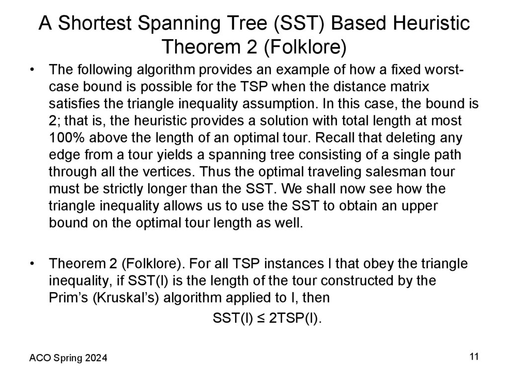
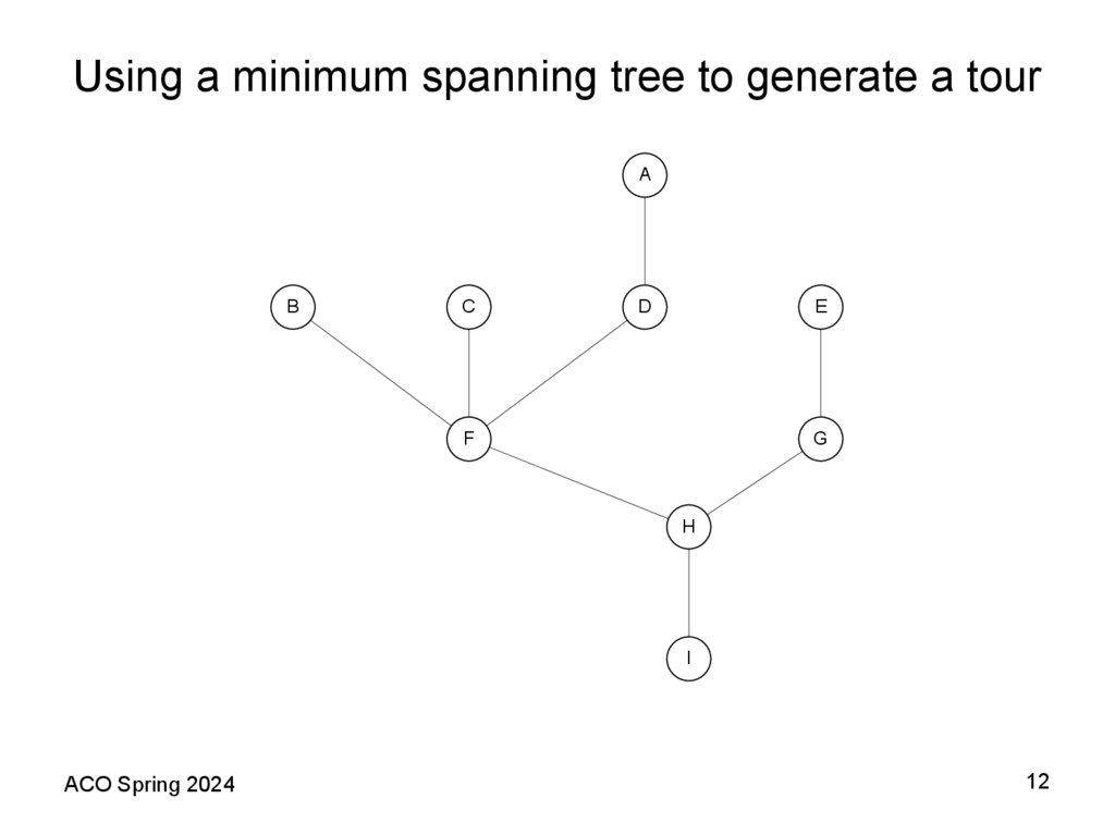
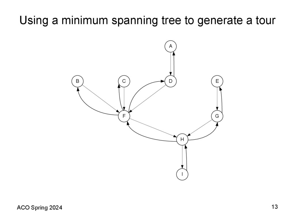
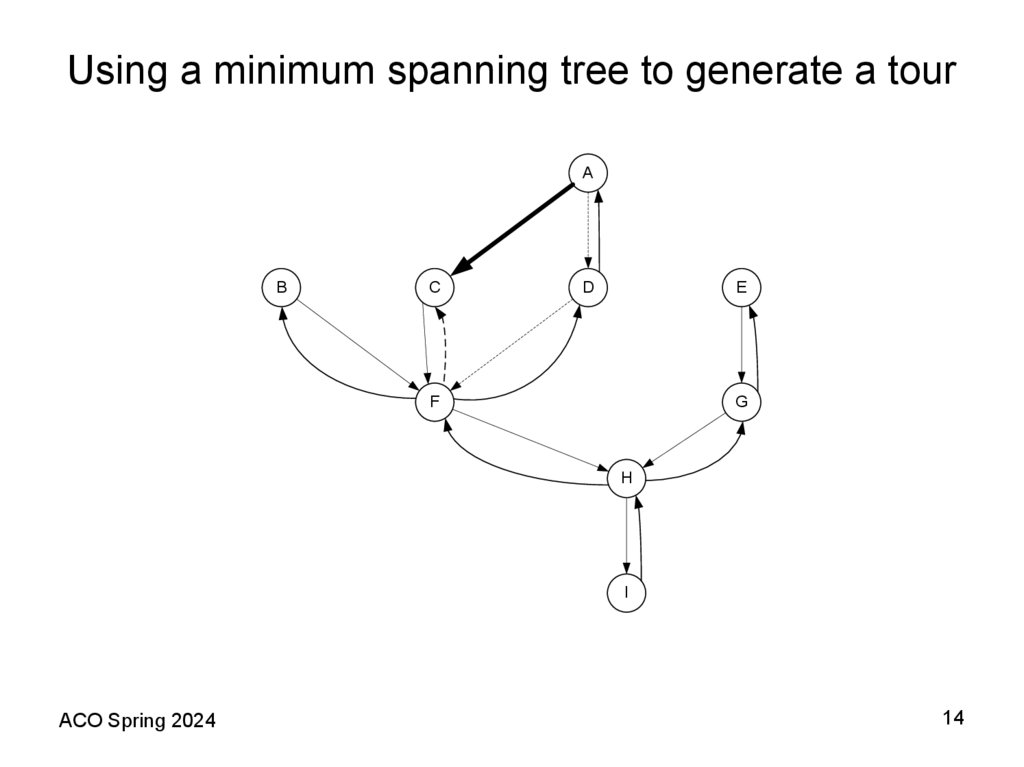
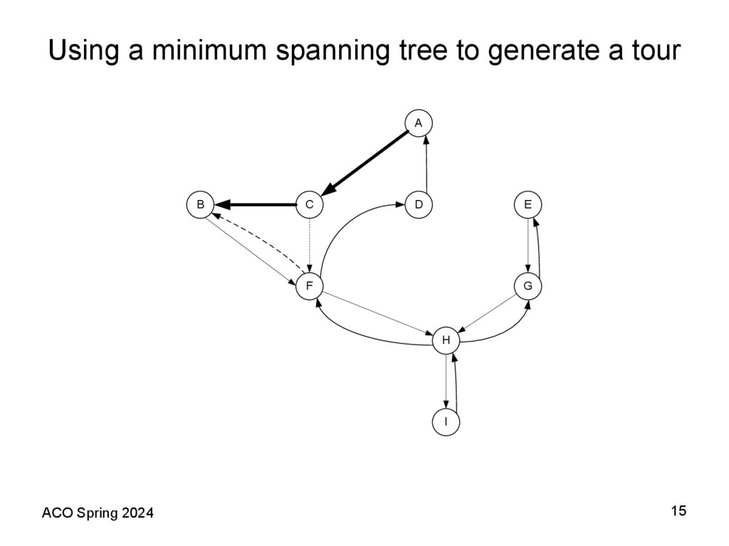
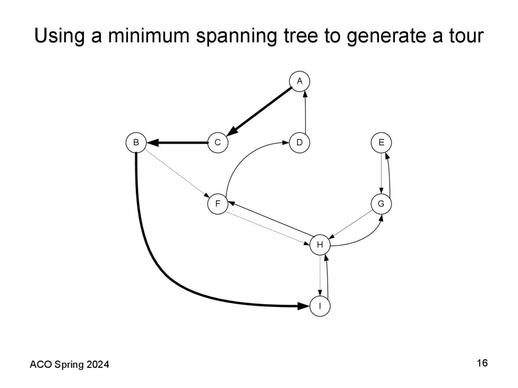
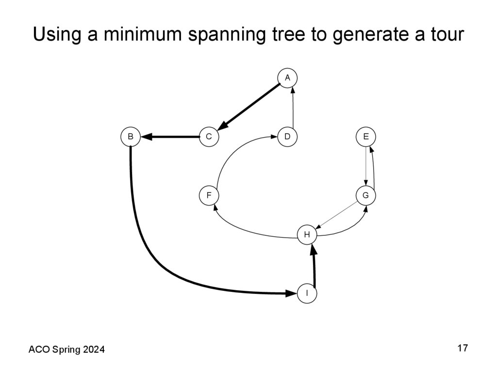
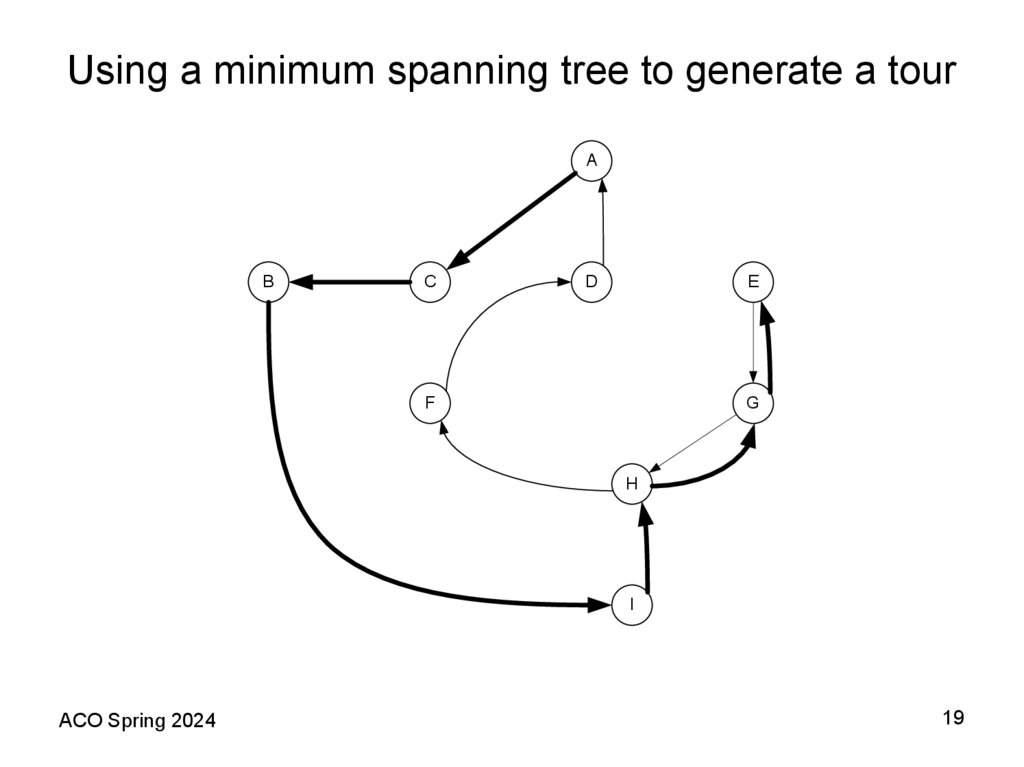
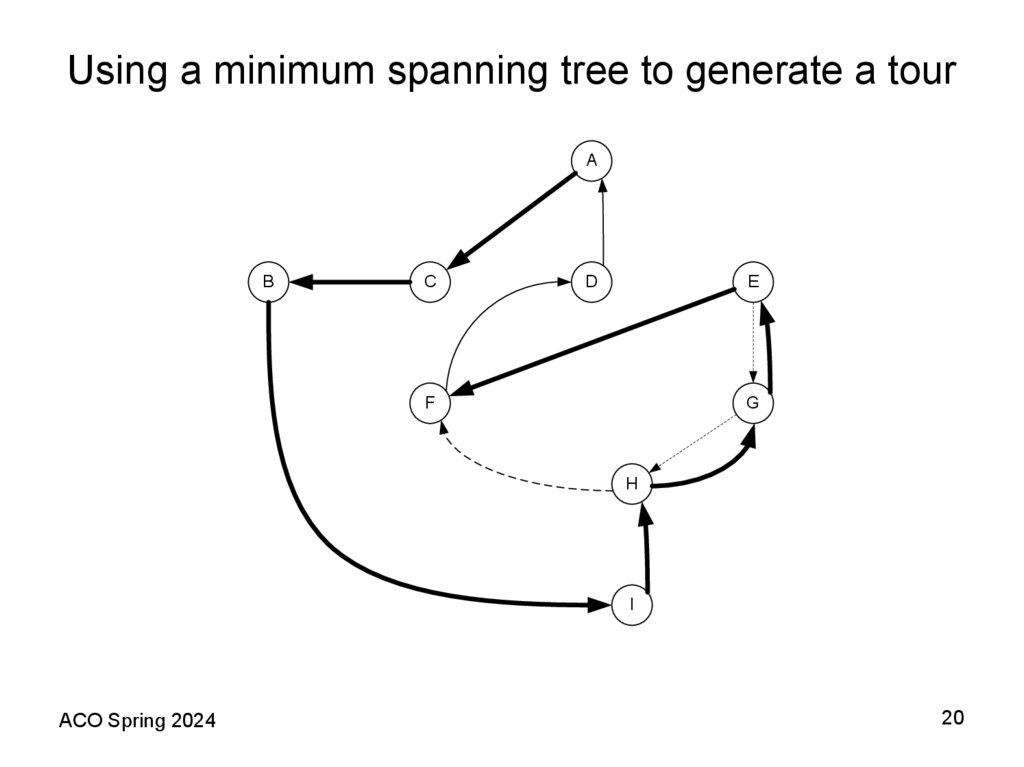
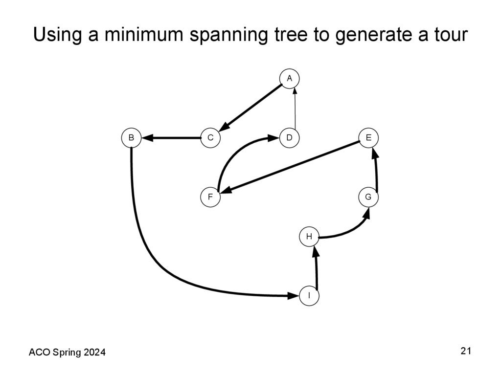
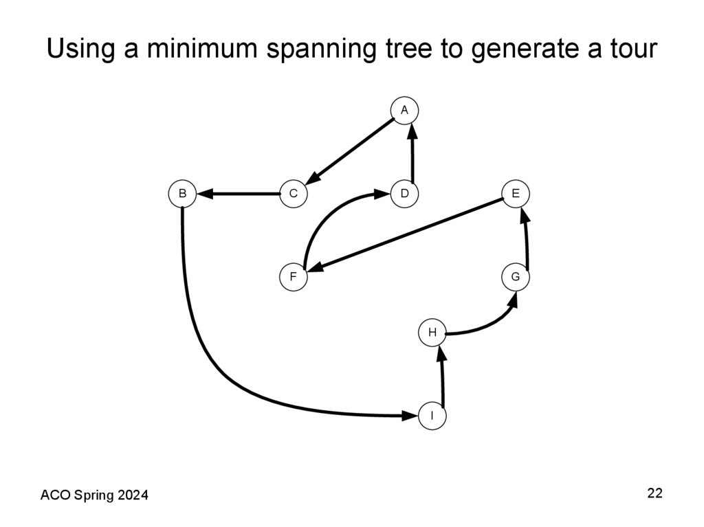
11. A Shortest Spanning Tree (SST) Based Heuristic Theorem 2 (Folklore)

• The following algorithm provides an example of how a fixed worstcase bound is possible for the TSP when the distance matrix
satisfies the triangle inequality assumption. In this case, the bound is
2; that is, the heuristic provides a solution with total length at most
100% above the length of an optimal tour. Recall that deleting any
edge from a tour yields a spanning tree consisting of a single path
through all the vertices. Thus the optimal traveling salesman tour
must be strictly longer than the SST. We shall now see how the
triangle inequality allows us to use the SST to obtain an upper
bound on the optimal tour length as well.
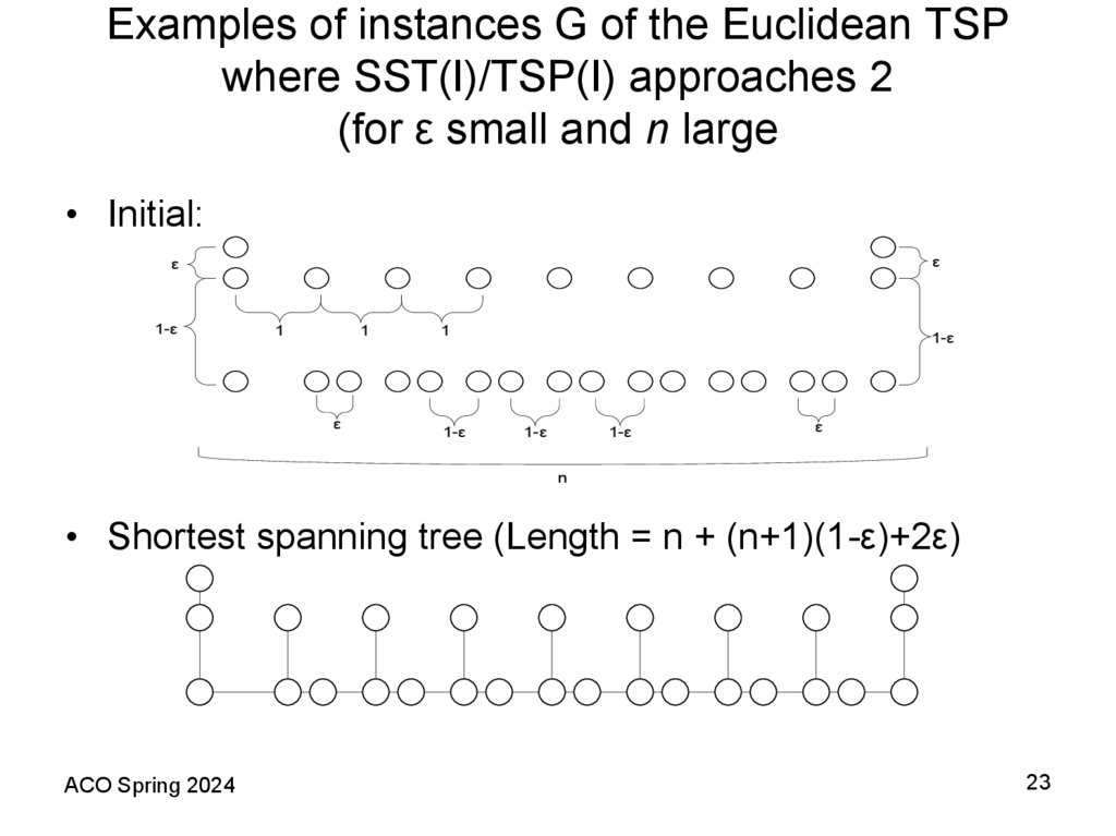
• Theorem 2 (Folklore). For all TSP instances I that obey the triangle
inequality, if SST(I) is the length of the tour constructed by the
Prim’s (Kruskal’s) algorithm applied to I, then
SST(I) ≤ 2TSP(I).
ACO Spring 2024
11

12. Using a minimum spanning tree to generate a tour

A
B
C
D
E
F
G
H
I
ACO Spring 2024
12

13. Using a minimum spanning tree to generate a tour

A
B
C
D
E
F
G
H
I
ACO Spring 2024
13

14. Using a minimum spanning tree to generate a tour

A
B
C
D
E
F
G
H
I
ACO Spring 2024
14

15. Using a minimum spanning tree to generate a tour

A
B
C
D
E
F
G
H
I
ACO Spring 2024
15

16. Using a minimum spanning tree to generate a tour

A
B
C
D
E
F
G
H
I
ACO Spring 2024
16

17. Using a minimum spanning tree to generate a tour

A
B
C
D
E
F
G
H
I
ACO Spring 2024
17

18. Using a minimum spanning tree to generate a tour

A
B
C
D
E
F
G
H
I
ACO Spring 2024
18

19. Using a minimum spanning tree to generate a tour

A
B
C
D
E
F
G
H
I
ACO Spring 2024
19

20. Using a minimum spanning tree to generate a tour

A
B
C
D
E
F
G
H
I
ACO Spring 2024
20

21. Using a minimum spanning tree to generate a tour

A
B
C
D
E
F
G
H
I
ACO Spring 2024
21

22. Using a minimum spanning tree to generate a tour

A
B
C
D
E
F
G
H
I
ACO Spring 2024
22

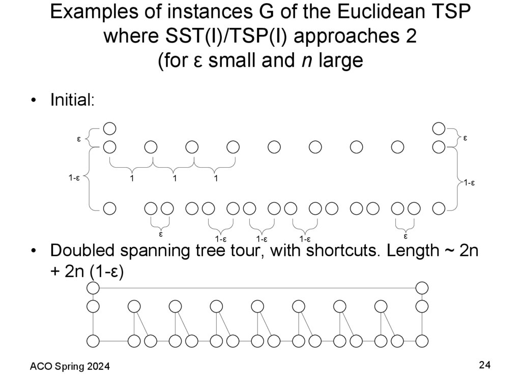
23. Examples of instances G of the Euclidean TSP where SST(I)/TSP(I) approaches 2 (for ε small and n large

• Initial:
ε
ε
1-ε
1
1
ε
1
1-ε
1-ε
1-ε
1-ε
ε
n
• Shortest spanning tree (Length = n + (n+1)(1-ε)+2ε)
ACO Spring 2024
23

24. Examples of instances G of the Euclidean TSP where SST(I)/TSP(I) approaches 2 (for ε small and n large

• Initial:
ε
ε
1-ε
1
1
ε
1
1-ε
1-ε
1-ε
1-ε
ε
• Doubled spanning tree tour, with shortcuts. Length ~ 2n
+ 2n (1-ε)
ACO Spring 2024
24

25. Examples of instances G of the Euclidean TSP where SST(I)/TSP(I) approaches 2 (for ε small and n large

• Initial:
ε
ε
1-ε
1
1
ε
1
1-ε
1-ε
1-ε
1-ε
ε
n
• Optimal tour, length ~ 2n + 2
ACO Spring 2024
25

26. Heuristic Algorithms for the TSP

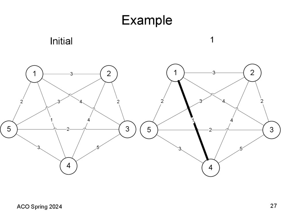
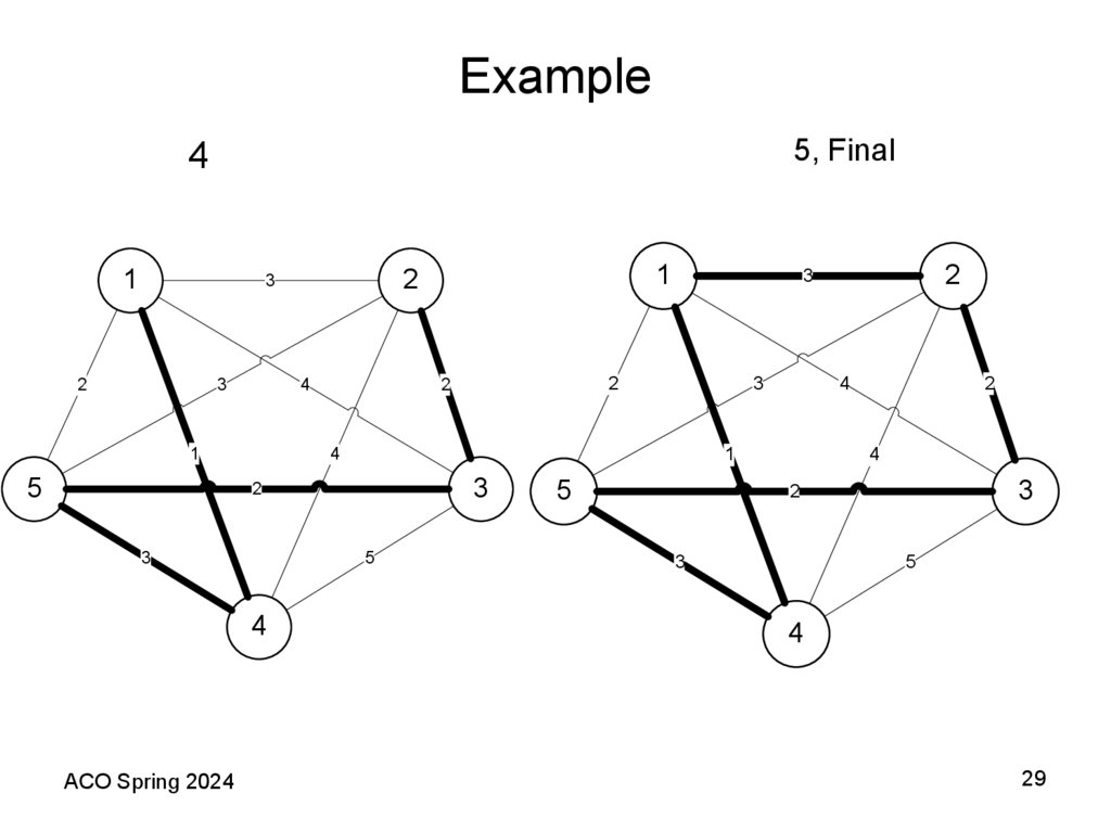
• Tour Construction Heuristic
A simple heuristic to build a tour is the nearest-neighbor
(NN) heuristic. This is essentially a greedy algorithm.
• Begin with any vertex x and find the vertex y so that c(x,
y) is the smallest among all y. Next, find the closest
vertex to y that is not already in the tour, say vertex z,
and add edge (y, z) to the tour. Repeat this process until
the last vertex is added and then join the first and last
vertices by the unique edge between them.
ACO Spring 2024
26

27. Example

1
Initial
1
2
3
4
1
5
3
4
3
5
4
4
1
3
2
3
2
2
2
ACO Spring 2024
1
2
3
5
2
4
3
2
3
5
4
27

28. Example

3
2
1
2
3
4
1
5
3
4
3
5
4
4
1
3
2
3
2
2
2
ACO Spring 2024
1
2
3
5
2
4
3
2
3
5
4
28

29. Example

5, Final
4
1
2
3
4
1
5
3
4
3
5
4
4
1
3
2
3
2
2
2
ACO Spring 2024
1
2
3
5
2
4
3
2
3
5
4
29

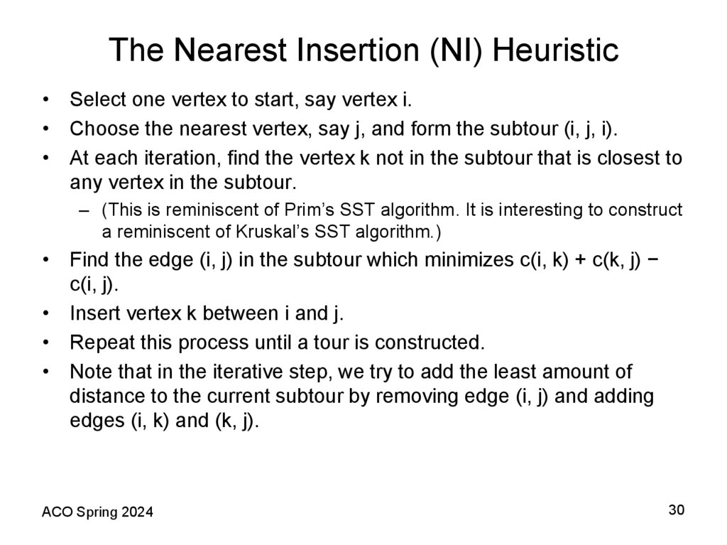
30. The Nearest Insertion (NI) Heuristic

• Select one vertex to start, say vertex i.
• Choose the nearest vertex, say j, and form the subtour (i, j, i).
• At each iteration, find the vertex k not in the subtour that is closest to
any vertex in the subtour.
– (This is reminiscent of Prim’s SST algorithm. It is interesting to construct
a reminiscent of Kruskal’s SST algorithm.)
• Find the edge (i, j) in the subtour which minimizes c(i, k) + c(k, j) −
c(i, j).
• Insert vertex k between i and j.
• Repeat this process until a tour is constructed.
• Note that in the iterative step, we try to add the least amount of
distance to the current subtour by removing edge (i, j) and adding
edges (i, k) and (k, j).
ACO Spring 2024
30

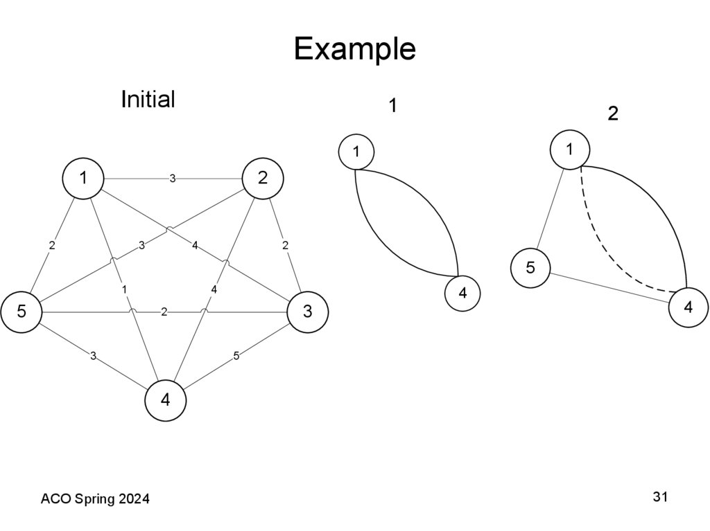
31. Example

Initial
1
2
1
1
1
2
3
2
3
4
2
5
1
5
4
4
3
4
3
2
5
4
ACO Spring 2024
31

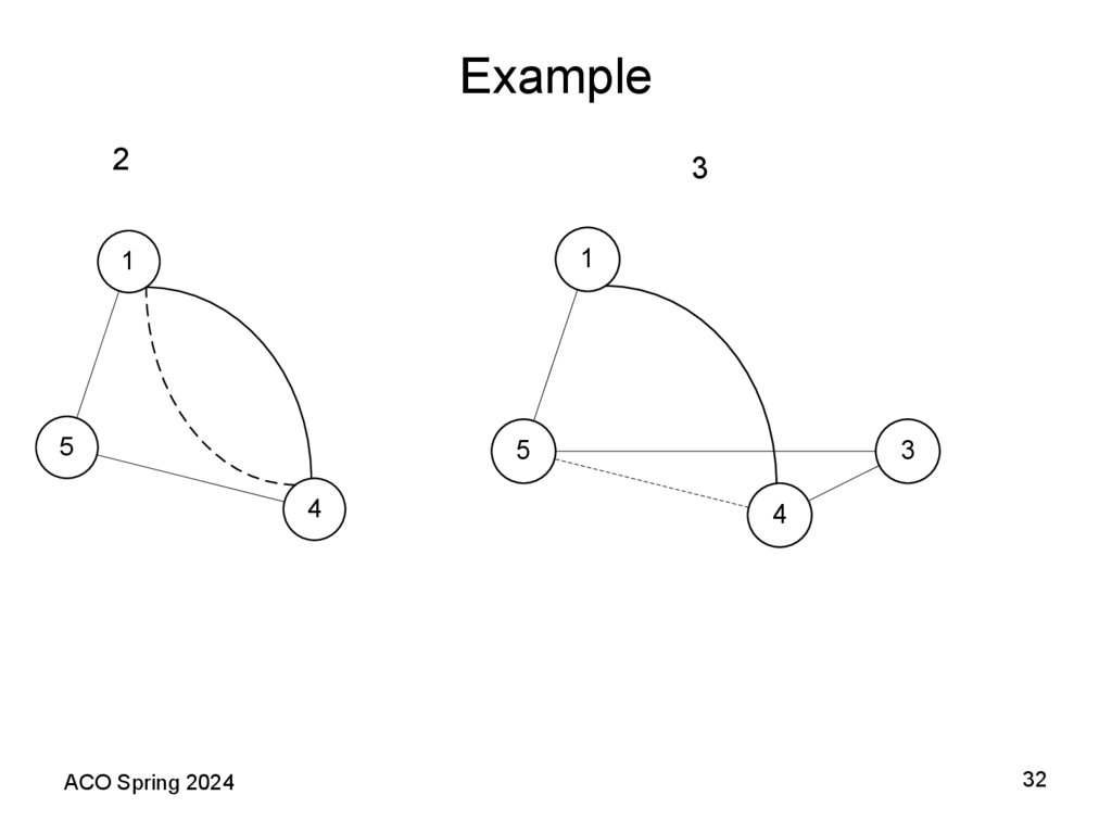
32. Example

2
3
1
1
5
5
4
ACO Spring 2024
3
4
32

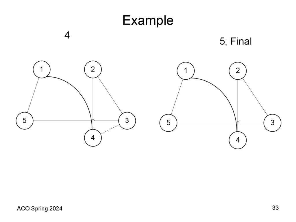
33. Example

4
1
5, Final
2
5
3
4
ACO Spring 2024
1
2
5
3
4
33

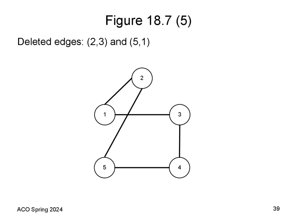
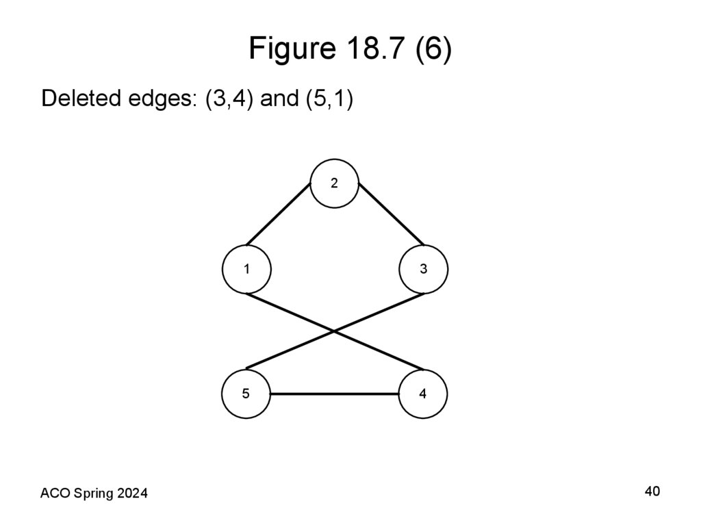
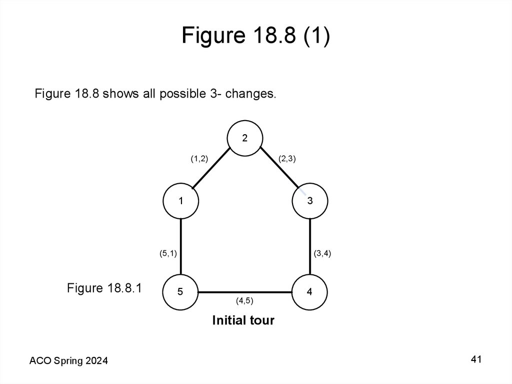
34. Tour Improvement Heuristics

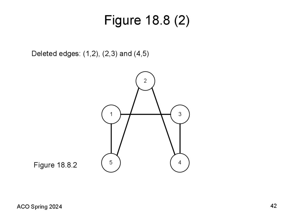
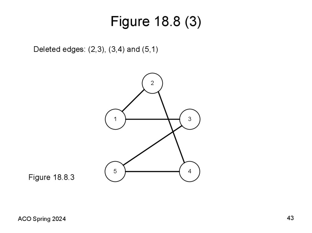
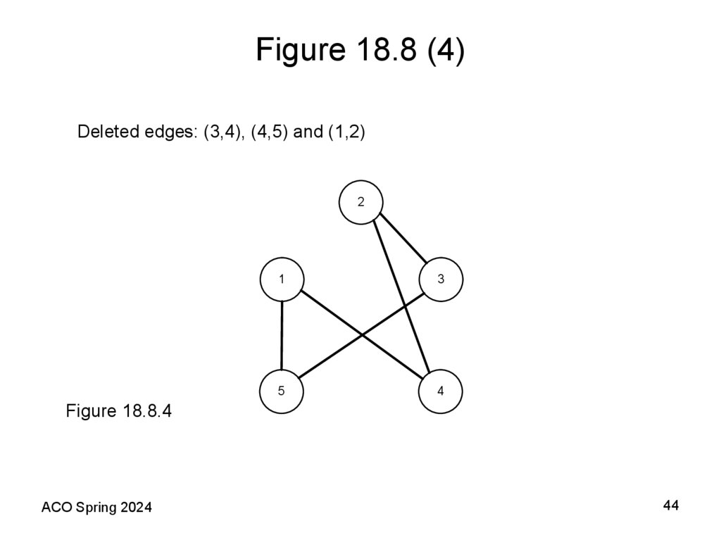
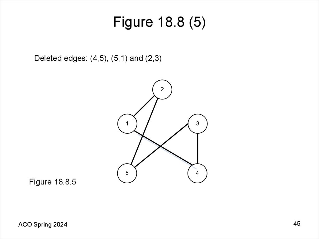
Some of the oldest and, by far, the most extensively used
heuristics developed for the TSP are so-called k-opt
heuristics (k ≥ 2). A k− change of a tour consists of
deleting k edges and replacing them by k other edges to
form a new tour.
ACO Spring 2024
34

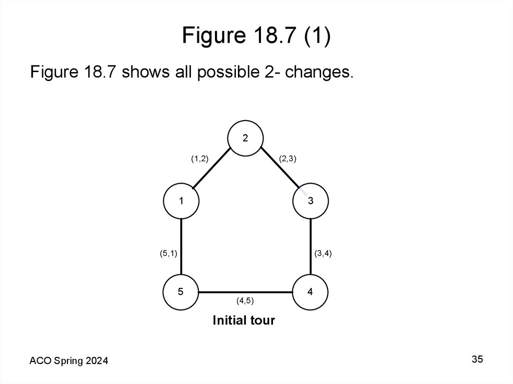
35. Figure 18.7 (1)

Figure 18.7 shows all possible 2- changes.
2
(1,2)
(2,3)
1
3
(5,1)
(3,4)
5
(4,5)
4
Initial tour
ACO Spring 2024
35

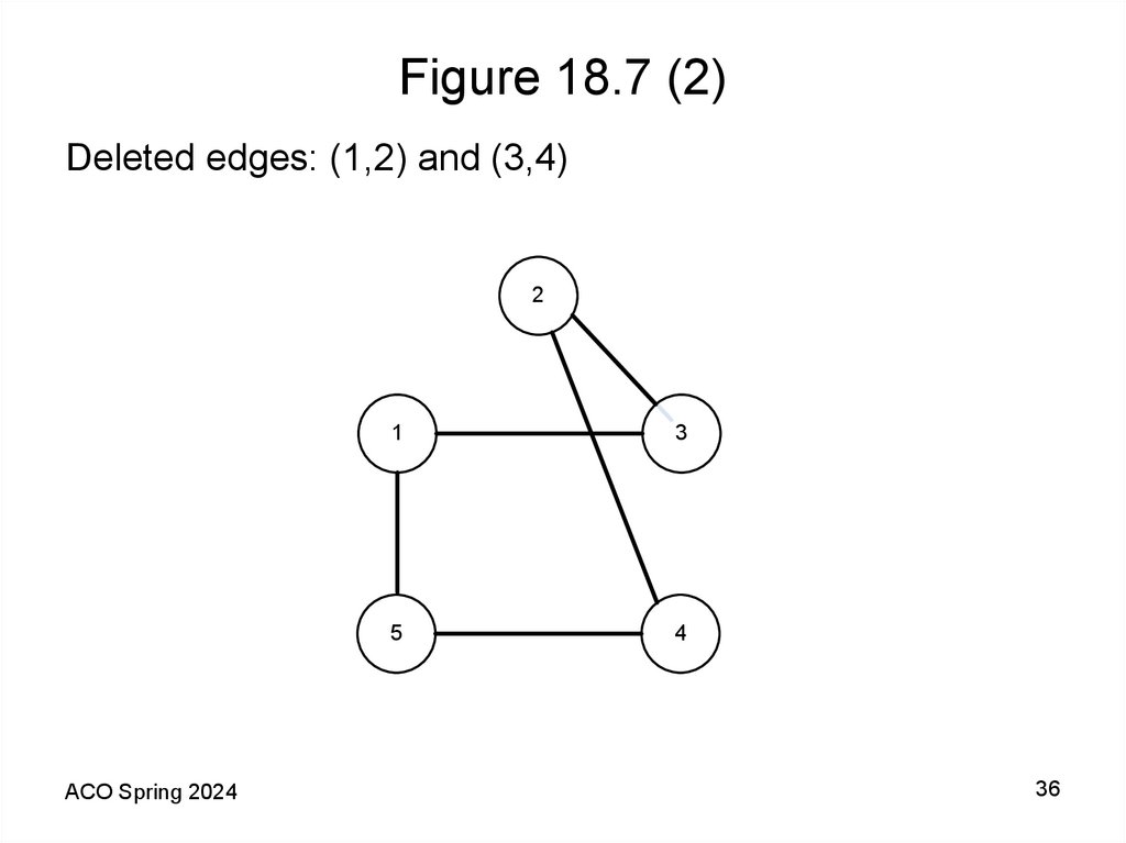
36. Figure 18.7 (2)

Deleted edges: (1,2) and (3,4)
2
ACO Spring 2024
1
3
5
4
36

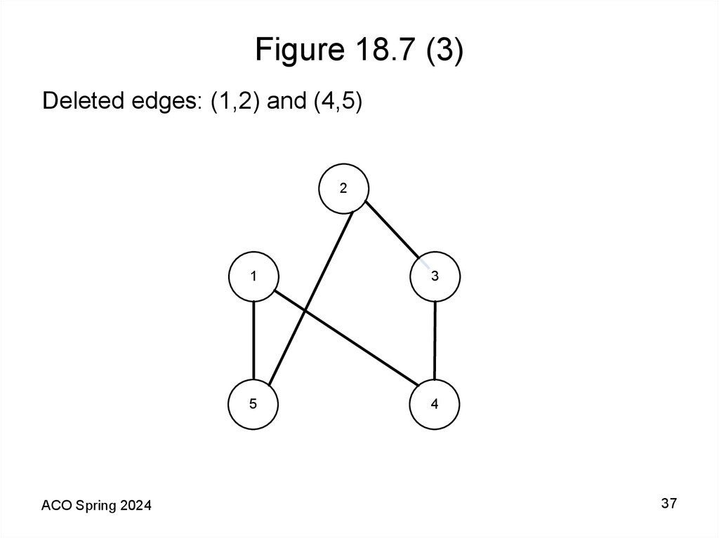
37. Figure 18.7 (3)

Deleted edges: (1,2) and (4,5)
2
ACO Spring 2024
1
3
5
4
37

38. Figure 18.7 (4)

Deleted edges: (2,3) and (4,5)
2
ACO Spring 2024
1
3
5
4
38

39. Figure 18.7 (5)

Deleted edges: (2,3) and (5,1)
2
ACO Spring 2024
1
3
5
4
39

40. Figure 18.7 (6)

Deleted edges: (3,4) and (5,1)
2
ACO Spring 2024
1
3
5
4
40

41. Figure 18.8 (1)

Figure 18.8 shows all possible 3- changes.
2
(1,2)
(2,3)
1
3
(5,1)
Figure 18.8.1
(3,4)
5
(4,5)
4
Initial tour
ACO Spring 2024
41

42. Figure 18.8 (2)

Deleted edges: (1,2), (2,3) and (4,5)
2
Figure 18.8.2
ACO Spring 2024
1
3
5
4
42

43. Figure 18.8 (3)

Deleted edges: (2,3), (3,4) and (5,1)
2
Figure 18.8.3
ACO Spring 2024
1
3
5
4
43

44. Figure 18.8 (4)

Deleted edges: (3,4), (4,5) and (1,2)
2
1
3
5
4
Figure 18.8.4
ACO Spring 2024
44

45. Figure 18.8 (5)

Deleted edges: (4,5), (5,1) and (2,3)
2
1
3
5
4
Figure 18.8.5
ACO Spring 2024
45

46. Figure 18.8 (6)

Deleted edges: (5,1), (1,2) and (3,4)
2
Figure 18.8.6
ACO Spring 2024
1
3
5
4
46

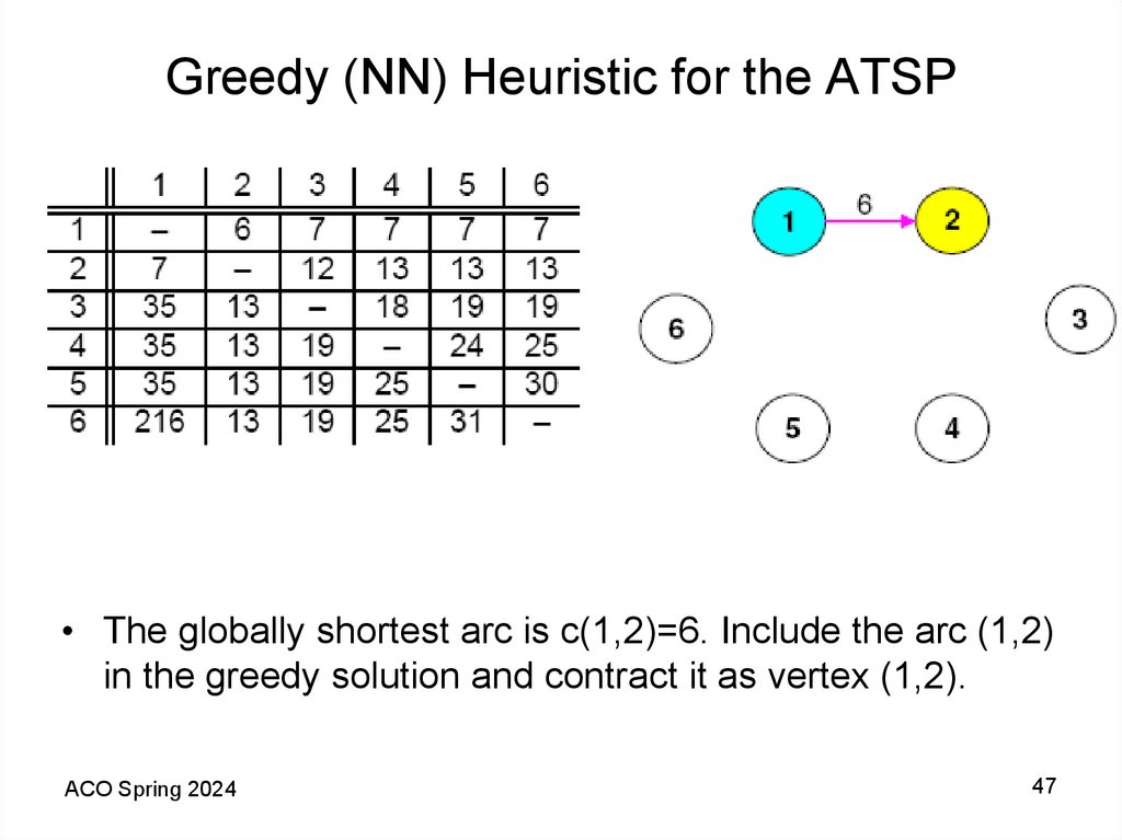
47. Greedy (NN) Heuristic for the ATSP

• The globally shortest arc is c(1,2)=6. Include the arc (1,2)
in the greedy solution and contract it as vertex (1,2).
ACO Spring 2024
47

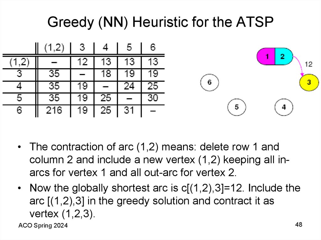
48. Greedy (NN) Heuristic for the ATSP

• The contraction of arc (1,2) means: delete row 1 and
column 2 and include a new vertex (1,2) keeping all inarcs for vertex 1 and all out-arc for vertex 2.
• Now the globally shortest arc is c[(1,2),3]=12. Include the
arc [(1,2),3] in the greedy solution and contract it as
vertex (1,2,3).
ACO Spring 2024
48

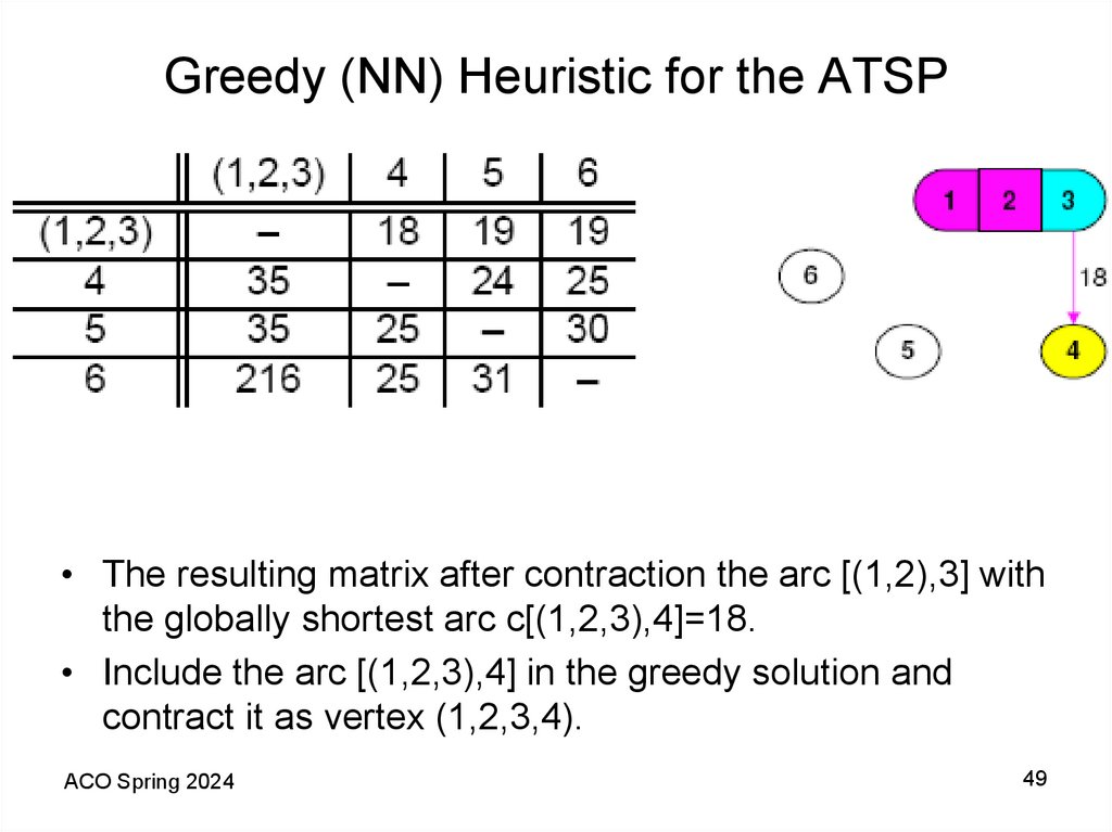
49. Greedy (NN) Heuristic for the ATSP

• The resulting matrix after contraction the arc [(1,2),3] with
the globally shortest arc c[(1,2,3),4]=18.
• Include the arc [(1,2,3),4] in the greedy solution and
contract it as vertex (1,2,3,4).
ACO Spring 2024
49

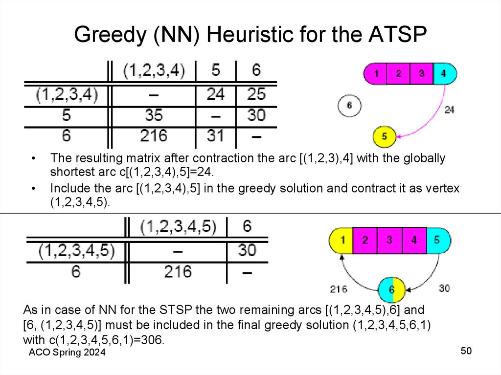
50. Greedy (NN) Heuristic for the ATSP

The resulting matrix after contraction the arc [(1,2,3),4] with the globally
shortest arc c[(1,2,3,4),5]=24.
Include the arc [(1,2,3,4),5] in the greedy solution and contract it as vertex
(1,2,3,4,5).
As in case of NN for the STSP the two remaining arcs [(1,2,3,4,5),6] and
[6, (1,2,3,4,5)] must be included in the final greedy solution (1,2,3,4,5,6,1)
with c(1,2,3,4,5,6,1)=306.
ACO Spring 2024
50

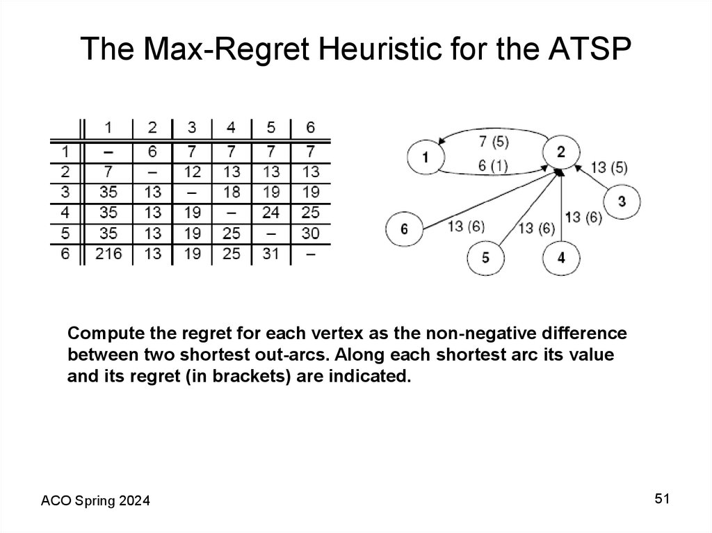
51. The Max-Regret Heuristic for the ATSP

1
Compute the regret for each vertex as the non-negative difference
between two shortest out-arcs. Along each shortest arc its value
and its regret (in brackets) are indicated.
ACO Spring 2024
51

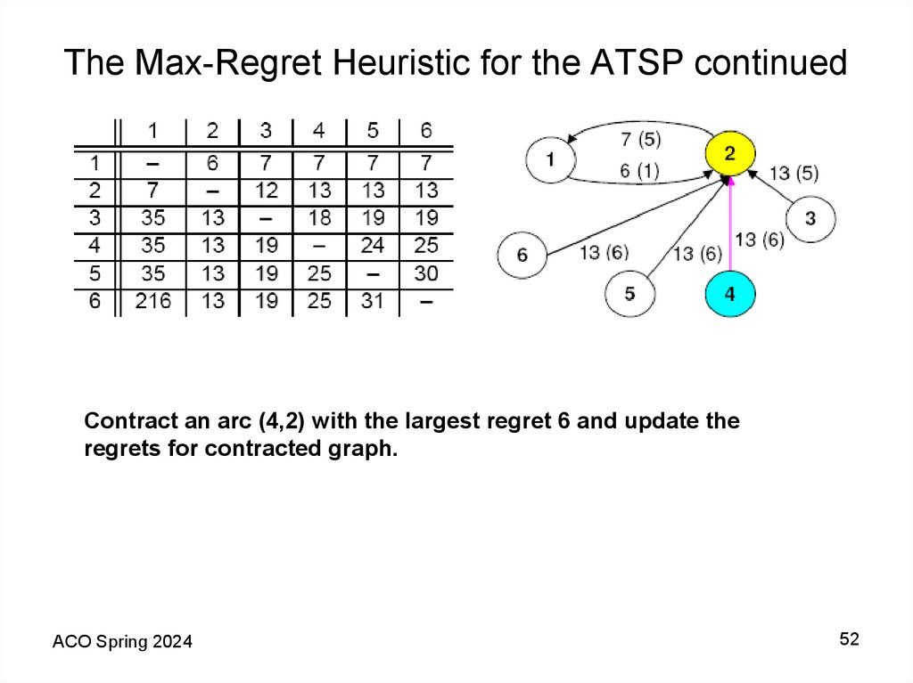
52. The Max-Regret Heuristic for the ATSP continued

1
Contract an arc (4,2) with the largest regret 6 and update the
regrets for contracted graph.
ACO Spring 2024
52

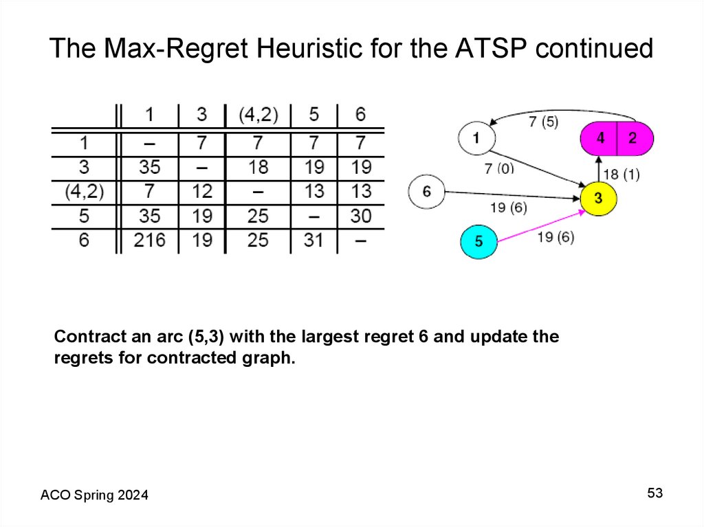
53. The Max-Regret Heuristic for the ATSP continued

Contract an arc (5,3) with the largest regret 6 and update the
regrets for contracted graph.
ACO Spring 2024
53

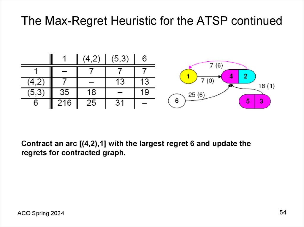
54. The Max-Regret Heuristic for the ATSP continued

Contract an arc [(4,2),1] with the largest regret 6 and update the
regrets for contracted graph.
ACO Spring 2024
54

55. The Max-Regret Heuristic for the ATSP continued

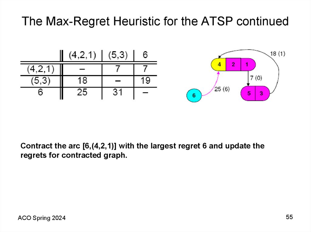
Contract the arc [6,(4,2,1)] with the largest regret 6 and update the
regrets for contracted graph.
ACO Spring 2024
55

56. The Max-Regret Heuristic for the ATSP continued

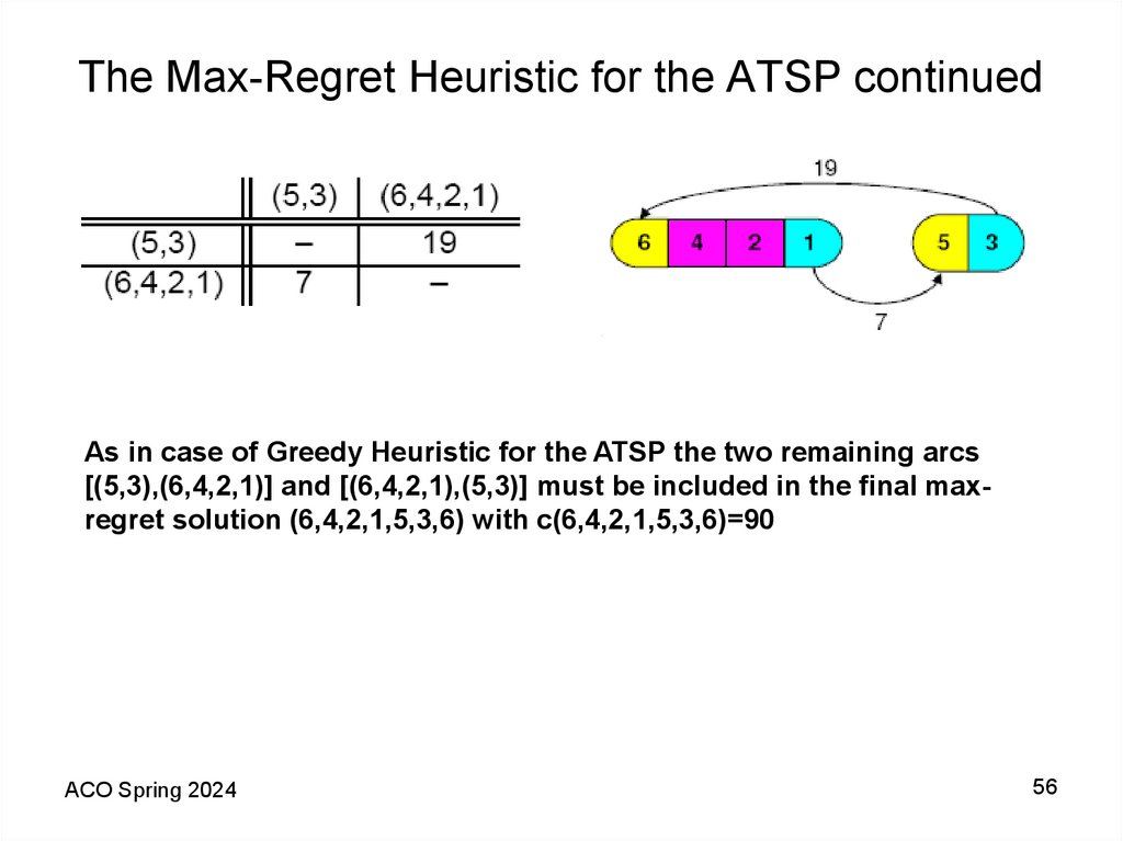
As in case of Greedy Heuristic for the ATSP the two remaining arcs
[(5,3),(6,4,2,1)] and [(6,4,2,1),(5,3)] must be included in the final maxregret solution (6,4,2,1,5,3,6) with c(6,4,2,1,5,3,6)=90
ACO Spring 2024
56

57. Summary

In this lecture, we examined the idea of using arc tolerances instead of
arc weights as a basis for making algorithmic decisions on whether or
not to include an arc in an optimal solution. Such methods have only
been studied in K. Helsgaun. An effective implementation of
the Lin-Kernighan traveling salesman heuristic. European Journal of
Operational Research 126, 106–130, 2000, and deserve more attention. In
order to evaluate the usefulness of the concept, three tolerance-based
greedy algorithms are proposed (see B. Goldengorin and G. Jager.How
To Make a Greedy Heuristic for the Asymmetric Traveling Salesman
Problem Competitive;
http://som.eldoc.ub.rug.nl/reports/themeA/2005/05A11/) for the ATSP.
Even though it needs time to calculate tolerances (in case of the
Max-Regret heuristic for each vertex just non-negative differences
between two shortest out-arcs), our computational experiments for the
wide range of ATSP instances show that tolerance based greedy
heuristics are much more accurate and faster than previously reported
greedy type algorithms.
ACO Spring 2024
57