Concepts and Techniques

1. Data Mining: Concepts and Techniques (3rd ed.) — Chapter 8 —

Jiawei Han, Micheline Kamber, and Jian Pei
University of Illinois at Urbana-Champaign &
Simon Fraser University
©2011 Han, Kamber & Pei. All rights reserved.
1

2.

3. Chapter 8. Classification: Basic Concepts

Classification: Basic Concepts
Decision Tree Induction
Bayes Classification Methods
Rule-Based Classification
Model Evaluation and Selection
Techniques to Improve Classification Accuracy:
Ensemble Methods
Summary
3

4. Supervised vs. Unsupervised Learning

Supervised learning (classification)
Supervision: The training data (observations,
measurements, etc.) are accompanied by labels indicating
the class of the observations
New data is classified based on the training set
Unsupervised learning (clustering)
The class labels of training data is unknown
Given a set of measurements, observations, etc. with the
aim of establishing the existence of classes or clusters in
the data
4

5. Prediction Problems: Classification vs. Numeric Prediction

Classification
predicts categorical class labels (discrete or nominal)
classifies data (constructs a model) based on the training
set and the values (class labels) in a classifying attribute
and uses it in classifying new data
Numeric Prediction
models continuous-valued functions, i.e., predicts
unknown or missing values
Typical applications
Credit/loan approval:
Medical diagnosis: if a tumor is cancerous or benign
Fraud detection: if a transaction is fraudulent
Web page categorization: which category it is
5

6. Classification—A Two-Step Process

Model construction: describing a set of predetermined classes
Each tuple/sample is assumed to belong to a predefined class, as
determined by the class label attribute
The set of tuples used for model construction is training set
The model is represented as classification rules, decision trees, or
mathematical formulae
Model usage: for classifying future or unknown objects
Estimate accuracy of the model
The known label of test sample is compared with the classified
result from the model
Accuracy rate is the percentage of test set samples that are
correctly classified by the model
Test set is independent of training set (otherwise overfitting)
If the accuracy is acceptable, use the model to classify new data
Note: If the test set is used to select models, it is called validation (test) set
6

7. Process (1): Model Construction

Training
Data
NAME RANK
YEARS TENURED
M ike
A ssistant P rof
3
no
M ary A ssistant P rof
7
yes
B ill
P rofessor
2
yes
Jim
A ssociate P rof
7
yes
D ave A ssistant P rof
6
no
A nne A ssociate P rof
3
no
Classification
Algorithms
Classifier
(Model)
IF rank = ‘professor’
OR years > 6
THEN tenured = ‘yes’
7

8. Process (2): Using the Model in Prediction

Classifier
Testing
Data
Unseen Data
(Jeff, Professor, 4)
NAME RANK
YEARS TENURED
T om
A ssistant P rof
2
no
M erlisa A ssociate P rof
7
no
G eorge P rofessor
5
yes
Joseph A ssistant P rof
7
yes
Tenured?
8

9. Chapter 8. Classification: Basic Concepts

Classification: Basic Concepts
Decision Tree Induction
Bayes Classification Methods
Rule-Based Classification
Model Evaluation and Selection
Techniques to Improve Classification Accuracy:
Ensemble Methods
Summary
9

10. Decision Tree Induction: An Example

Training data set: Buys_computer
The data set follows an example of
Quinlan’s ID3 (Playing Tennis)
Resulting tree:
age?
<=30
31..40
overcast
student?
no
no
yes
yes
yes
>40
age income student credit_rating buys_computer
<=30
high
no fair
no
<=30
high
no excellent
no
31…40 high
no fair
yes
>40
medium
no fair
yes
>40
low
yes fair
yes
>40
low
yes excellent
no
31…40 low
yes excellent
yes
<=30
medium
no fair
no
<=30
low
yes fair
yes
>40
medium yes fair
yes
<=30
medium yes excellent
yes
31…40 medium
no excellent
yes
31…40 high
yes fair
yes
>40
medium
no excellent
no
credit rating?
excellent
fair
yes
10

11. Algorithm for Decision Tree Induction

Basic algorithm (a greedy algorithm)
Tree is constructed in a top-down recursive divide-andconquer manner
At start, all the training examples are at the root
Attributes are categorical (if continuous-valued, they are
discretized in advance)
Examples are partitioned recursively based on selected
attributes
Test attributes are selected on the basis of a heuristic or
statistical measure (e.g., information gain)
Conditions for stopping partitioning
All samples for a given node belong to the same class
There are no remaining attributes for further partitioning –
majority voting is employed for classifying the leaf
There are no samples left
11

12. Brief Review of Entropy

m=2
12

13.

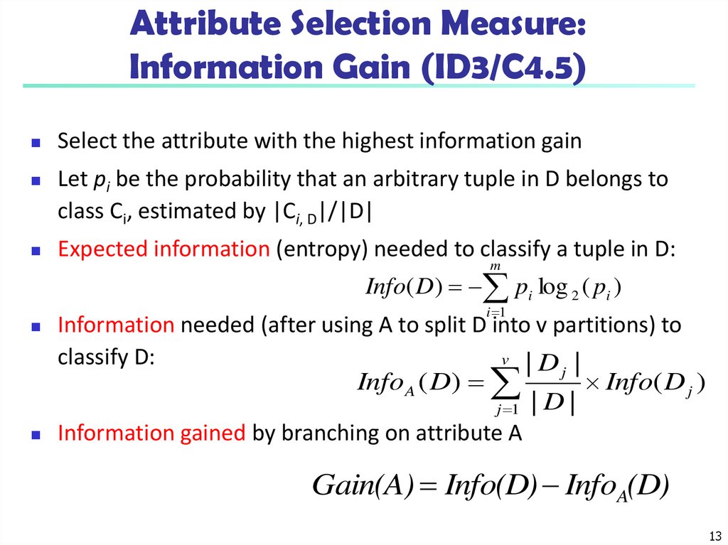
Attribute Selection Measure:
Information Gain (ID3/C4.5)
Select the attribute with the highest information gain
Let pi be the probability that an arbitrary tuple in D belongs to
class Ci, estimated by |Ci, D|/|D|
Expected information (entropy) needed to classify a tuple in D:
m
Info( D) pi log 2 ( pi )
i 1
Information needed (after using A to split D into v partitions) to
v | D |
classify D:
j
InfoA ( D)
Info( D j )
j 1 | D |
Information gained by branching on attribute A
Gain(A) Info(D) InfoA(D)
13

14. Attribute Selection: Information Gain

Class P: buys_computer = “yes”
Infoage ( D )
Class N: buys_computer = “no”
Info( D) I (9,5)
age
<=30
31…40
>40
age
<=30
<=30
31…40
>40
>40
>40
31…40
<=30
<=30
>40
<=30
31…40
31…40
>40
9
9
5
5
log 2 ( ) log 2 ( ) 0.940
14
14 14
14
pi
2
4
3
ni I(pi, ni)
3 0.971
0 0
2 0.971
income student credit_rating
high
no
fair
high
no
excellent
high
no
fair
medium
no
fair
low
yes fair
low
yes excellent
low
yes excellent
medium
no
fair
low
yes fair
medium
yes fair
medium
yes excellent
medium
no
excellent
high
yes fair
medium
no
excellent
buys_computer
no
no
yes
yes
yes
no
yes
no
yes
yes
yes
yes
yes
no
5
4
I (2,3)
I ( 4,0)
14
14
5
I (3,2) 0.694
14
5
I ( 2,3)means “age <=30” has 5 out of
14
14 samples, with 2 yes’es and 3
no’s. Hence
Gain(age) Info( D) Infoage ( D) 0.246
Similarly,
Gain(income) 0.029
Gain( student ) 0.151
Gain(credit _ rating ) 0.048
14

15. Computing Information-Gain for Continuous-Valued Attributes

Let attribute A be a continuous-valued attribute
Must determine the best split point for A
Sort the value A in increasing order
Typically, the midpoint between each pair of adjacent values
is considered as a possible split point
(ai+ai+1)/2 is the midpoint between the values of ai and ai+1
The point with the minimum expected information
requirement for A is selected as the split-point for A
Split:
D1 is the set of tuples in D satisfying A ≤ split-point, and D2 is
the set of tuples in D satisfying A > split-point
15

16. Gain Ratio for Attribute Selection (C4.5)

Information gain measure is biased towards attributes with a
large number of values
C4.5 (a successor of ID3) uses gain ratio to overcome the
problem (normalization to information gain)
v
SplitInfo A ( D)
j 1
| Dj |
|D|
log 2 (
| Dj |
|D|
)
GainRatio(A) = Gain(A)/SplitInfo(A)
Ex.
gain_ratio(income) = 0.029/1.557 = 0.019
The attribute with the maximum gain ratio is selected as the
splitting attribute
16

17. Gini Index (CART, IBM IntelligentMiner)

If a data set D contains examples from n classes, gini index,
n
gini(D) is defined as
2
gini( D) 1 p j
j 1
where pj is the relative frequency of class j in D
If a data set D is split on A into two subsets D1 and D2, the gini
index gini(D) is defined as
gini A (D)
|D1|
|D |
gini(D1) 2 gini(D2)
|D|
|D|
Reduction in Impurity:
The attribute provides the smallest ginisplit(D) (or the largest
reduction in impurity) is chosen to split the node (need to
enumerate all the possible splitting points for each attribute)
gini( A) gini(D) giniA (D)
17

18. Computation of Gini Index

Ex. D has 9 tuples in buys_computer = “yes”
and
5 in “no”
2
2
9 5
gini ( D) 1 0.459
14 14
Suppose the attribute income partitions D into 10 in D1: {low,
medium} and 4 in D2 giniincome {low,medium} ( D) 10 Gini( D1 ) 4 Gini( D2 )
14
14
Gini{low,high} is 0.458; Gini{medium,high} is 0.450. Thus, split on the
{low,medium} (and {high}) since it has the lowest Gini index
All attributes are assumed continuous-valued
May need other tools, e.g., clustering, to get the possible split
values
Can be modified for categorical attributes
18

19. Comparing Attribute Selection Measures

The three measures, in general, return good results but
Information gain:
Gain ratio:
biased towards multivalued attributes
tends to prefer unbalanced splits in which one partition is
much smaller than the others
Gini index:
biased to multivalued attributes
has difficulty when # of classes is large
tends to favor tests that result in equal-sized partitions
and purity in both partitions
19

20. Other Attribute Selection Measures

CHAID: a popular decision tree algorithm, measure based on χ2 test for
independence
C-SEP: performs better than info. gain and gini index in certain cases
G-statistic: has a close approximation to χ2 distribution
MDL (Minimal Description Length) principle (i.e., the simplest solution is
preferred):
The best tree as the one that requires the fewest # of bits to both (1)
encode the tree, and (2) encode the exceptions to the tree
Multivariate splits (partition based on multiple variable combinations)
CART: finds multivariate splits based on a linear comb. of attrs.
Which attribute selection measure is the best?
Most give good results, none is significantly superior than others
20

21. Overfitting and Tree Pruning

Overfitting: An induced tree may overfit the training data
Too many branches, some may reflect anomalies due to
noise or outliers
Poor accuracy for unseen samples
Two approaches to avoid overfitting
Prepruning: Halt tree construction early ̵ do not split a node
if this would result in the goodness measure falling below a
threshold
Difficult to choose an appropriate threshold
Postpruning: Remove branches from a “fully grown” tree—
get a sequence of progressively pruned trees
Use a set of data different from the training data to
decide which is the “best pruned tree”
21

22. Enhancements to Basic Decision Tree Induction

Bayesian Classification: Why?
A statistical classifier: performs probabilistic prediction, i.e.,
predicts class membership probabilities
Foundation: Based on Bayes’ Theorem.
Performance: A simple Bayesian classifier, naïve Bayesian
classifier, has comparable performance with decision tree and
selected neural network classifiers
Incremental: Each training example can incrementally
increase/decrease the probability that a hypothesis is correct —
prior knowledge can be combined with observed data
Standard: Even when Bayesian methods are computationally
intractable, they can provide a standard of optimal decision
making against which other methods can be measured
31

23. Classification in Large Databases

Bayes’ Theorem: Basics
M
Total probability Theorem: P(B) P(B | Ai )P( Ai )
Bayes’ Theorem: P(H | X) P(X | H )P(H ) P(X | H ) P(H ) / P(X)
i 1
P(X)
Let X be a data sample (“evidence”): class label is unknown
Let H be a hypothesis that X belongs to class C
Classification is to determine P(H|X), (i.e., posteriori probability): the
probability that the hypothesis holds given the observed data sample X
P(H) (prior probability): the initial probability
E.g., X will buy computer, regardless of age, income, …
P(X): probability that sample data is observed
P(X|H) (likelihood): the probability of observing the sample X, given that
the hypothesis holds
E.g., Given that X will buy computer, the prob. that X is 31..40,
medium income
32

24. Scalability Framework for RainForest

Prediction Based on Bayes’ Theorem
Given training data X, posteriori probability of a hypothesis H,
P(H|X), follows the Bayes’ theorem
P(H | X) P(X | H )P(H ) P(X | H ) P(H ) / P(X)
P(X)
Informally, this can be viewed as
posteriori = likelihood x prior/evidence
Predicts X belongs to Ci iff the probability P(Ci|X) is the highest
among all the P(Ck|X) for all the k classes
Practical difficulty: It requires initial knowledge of many
probabilities, involving significant computational cost
33

25. Rainforest: Training Set and Its AVC Sets

Classification Is to Derive the Maximum Posteriori
Let D be a training set of tuples and their associated class
labels, and each tuple is represented by an n-D attribute vector
X = (x1, x2, …, xn)
Suppose there are m classes C1, C2, …, Cm.
Classification is to derive the maximum posteriori, i.e., the
maximal P(Ci|X)
This can be derived from Bayes’ theorem
P(X | C )P(C )
i
i
P(C | X)
i
P(X)
Since P(X) is constant for all classes, only
P(C | X) P(X | C )P(C )
i
i
i
needs to be maximized
34

26. BOAT (Bootstrapped Optimistic Algorithm for Tree Construction)

Naïve Bayes Classifier
A simplified assumption: attributes are conditionally
independent (i.e., no dependence relation between
n
attributes):
P( X | C i ) P( x | C i) P( x | C i) P( x | C i) ... P( x | C i)
k
1
2
n
k 1
This greatly reduces the computation cost: Only counts the
class distribution
If Ak is categorical, P(xk|Ci) is the # of tuples in Ci having value xk
for Ak divided by |Ci, D| (# of tuples of Ci in D)
If Ak is continous-valued, P(xk|Ci) is usually computed based on
Gaussian distribution with a mean μ and standard deviation σ
and P(xk|Ci) is
g ( x, , )
1
e
2
( x )2
2 2
P ( X | C i ) g ( xk , Ci , C i )
35

27.

Naïve Bayes Classifier: Training Dataset
Class:
C1:buys_computer = ‘yes’
C2:buys_computer = ‘no’
Data to be classified:
X = (age <=30,
Income = medium,
Student = yes
Credit_rating = Fair)
age
<=30
<=30
31…40
>40
>40
>40
31…40
<=30
<=30
>40
<=30
31…40
31…40
>40
income studentcredit_rating
buys_compu
high
no fair
no
high
no excellent
no
high
no fair
yes
medium no fair
yes
low
yes fair
yes
low
yes excellent
no
low
yes excellent yes
medium no fair
no
low
yes fair
yes
medium yes fair
yes
medium yes excellent yes
medium no excellent yes
high
yes fair
yes
medium no excellent
no
36

28. Visualization of a Decision Tree in SGI/MineSet 3.0

Naïve Bayes Classifier: An Example
age
<=30
<=30
31…40
>40
>40
>40
31…40
<=30
<=30
>40
<=30
31…40
31…40
>40
income studentcredit_rating
buys_comp
high
no fair
no
high
no excellent
no
high
no fair
yes
medium
no fair
yes
low
yes fair
yes
low
yes excellent
no
low
yes excellent
yes
medium
no fair
no
low
yes fair
yes
medium yes fair
yes
medium yes excellent
yes
medium
no excellent
yes
high
yes fair
yes
medium
no excellent
no
P(Ci): P(buys_computer = “yes”) = 9/14 = 0.643
P(buys_computer = “no”) = 5/14= 0.357
Compute P(X|Ci) for each class
P(age = “<=30” | buys_computer = “yes”) = 2/9 = 0.222
P(age = “<= 30” | buys_computer = “no”) = 3/5 = 0.6
P(income = “medium” | buys_computer = “yes”) = 4/9 = 0.444
P(income = “medium” | buys_computer = “no”) = 2/5 = 0.4
P(student = “yes” | buys_computer = “yes) = 6/9 = 0.667
P(student = “yes” | buys_computer = “no”) = 1/5 = 0.2
P(credit_rating = “fair” | buys_computer = “yes”) = 6/9 = 0.667
P(credit_rating = “fair” | buys_computer = “no”) = 2/5 = 0.4
X = (age <= 30 , income = medium, student = yes, credit_rating = fair)
P(X|Ci) : P(X|buys_computer = “yes”) = 0.222 x 0.444 x 0.667 x 0.667 = 0.044
P(X|buys_computer = “no”) = 0.6 x 0.4 x 0.2 x 0.4 = 0.019
P(X|Ci)*P(Ci) : P(X|buys_computer = “yes”) * P(buys_computer = “yes”) = 0.028
P(X|buys_computer = “no”) * P(buys_computer = “no”) = 0.007
Therefore, X belongs to class (“buys_computer = yes”)
37

29. Interactive Visual Mining by Perception-Based Classification (PBC)

Avoiding the Zero-Probability Problem
Naïve Bayesian prediction requires each conditional prob. be
non-zero. Otherwise, the predicted prob. will be zero
P( X | C i)
n
P( x k | C i)
k 1
Ex. Suppose a dataset with 1000 tuples, income=low (0),
income= medium (990), and income = high (10)
Use Laplacian correction (or Laplacian estimator)
Adding 1 to each case
Prob(income = low) = 1/1003
Prob(income = medium) = 991/1003
Prob(income = high) = 11/1003
The “corrected” prob. estimates are close to their
“uncorrected” counterparts
38

30. Chapter 8. Classification: Basic Concepts

Naïve Bayes Classifier: Comments
Advantages
Easy to implement
Good results obtained in most of the cases
Disadvantages
Assumption: class conditional independence, therefore loss
of accuracy
Practically, dependencies exist among variables
E.g., hospitals: patients: Profile: age, family history, etc.
Symptoms: fever, cough etc., Disease: lung cancer,
diabetes, etc.
Dependencies among these cannot be modeled by Naïve
Bayes Classifier
How to deal with these dependencies? Bayesian Belief Networks
(Chapter 9)
39

31. Bayesian Classification: Why?

Chapter 8. Classification: Basic Concepts
Classification: Basic Concepts
Decision Tree Induction
Bayes Classification Methods
Rule-Based Classification
Model Evaluation and Selection
Techniques to Improve Classification Accuracy:
Ensemble Methods
Summary
47

32. Bayes’ Theorem: Basics

Model Evaluation and Selection
Evaluation metrics: How can we measure accuracy? Other
metrics to consider?
Use validation test set of class-labeled tuples instead of
training set when assessing accuracy
Methods for estimating a classifier’s accuracy:
Holdout method, random subsampling
Cross-validation
Bootstrap
Comparing classifiers:
Confidence intervals
Cost-benefit analysis and ROC Curves
48

33. Prediction Based on Bayes’ Theorem

Classifier Evaluation Metrics: Confusion
Matrix
Confusion Matrix:
Actual class\Predicted class
C1
¬ C1
C1
True Positives (TP)
False Negatives (FN)
¬ C1
False Positives (FP)
True Negatives (TN)
Example of Confusion Matrix:
Actual class\Predicted buy_computer buy_computer
class
= yes
= no
Total
buy_computer = yes
6954
46
7000
buy_computer = no
412
2588
3000
Total
7366
2634
10000
Given m classes, an entry, CMi,j in a confusion matrix indicates
# of tuples in class i that were labeled by the classifier as class j
May have extra rows/columns to provide totals
49

34. Classification Is to Derive the Maximum Posteriori

Classifier Evaluation Metrics: Accuracy,
Error Rate, Sensitivity and Specificity
A\P
C
¬C
Class Imbalance Problem:
C TP FN P
One class may be rare, e.g.
¬C FP TN N
fraud, or HIV-positive
P’ N’ All
Significant majority of the
negative class and minority of
Classifier Accuracy, or
the positive class
recognition rate: percentage of
test set tuples that are correctly Sensitivity: True Positive
classified
recognition rate
Accuracy = (TP + TN)/All
Sensitivity = TP/P
Error rate: 1 – accuracy, or
Specificity: True Negative
recognition rate
Error rate = (FP + FN)/All
Specificity = TN/N
50

35. Naïve Bayes Classifier

Classifier Evaluation Metrics:
Precision and Recall, and F-measures
Precision: exactness – what % of tuples that the classifier
labeled as positive are actually positive
Recall: completeness – what % of positive tuples did the
classifier label as positive?
Perfect score is 1.0
Inverse relationship between precision & recall
F measure (F1 or F-score): harmonic mean of precision and
recall,
Fß: weighted measure of precision and recall
assigns ß times as much weight to recall as to precision
51

36. Naïve Bayes Classifier: Training Dataset

Classifier Evaluation Metrics: Example
Actual Class\Predicted class
cancer = yes
cancer = no
Total
Recognition(%)
cancer = yes
90
210
300
30.00 (sensitivity
cancer = no
140
9560
9700
98.56 (specificity)
Total
230
9770
10000
96.40 (accuracy)
Precision = 90/230 = 39.13%
Recall = 90/300 = 30.00%
52