Cmpe 466 computer graphics. 2d geometric transformations. (Chapter 7)

1. CMPE 466 COMPUTER GRAPHICS

1
CMPE 466
COMPUTER GRAPHICS
Chapter 7
2D Geometric Transformations
Instructor: D. Arifler
Material based on
- Computer Graphics with OpenGL®, Fourth Edition by Donald Hearn, M. Pauline Baker, and Warren R. Carithers
- Fundamentals of Computer Graphics, Third Edition by by Peter Shirley and Steve Marschner
- Computer Graphics by F. S. Hill

2. Basic geometric transformations

2
Basic geometric transformations
• Translation
• Rotation
• Scaling

3. 2D translation

3
2D translation
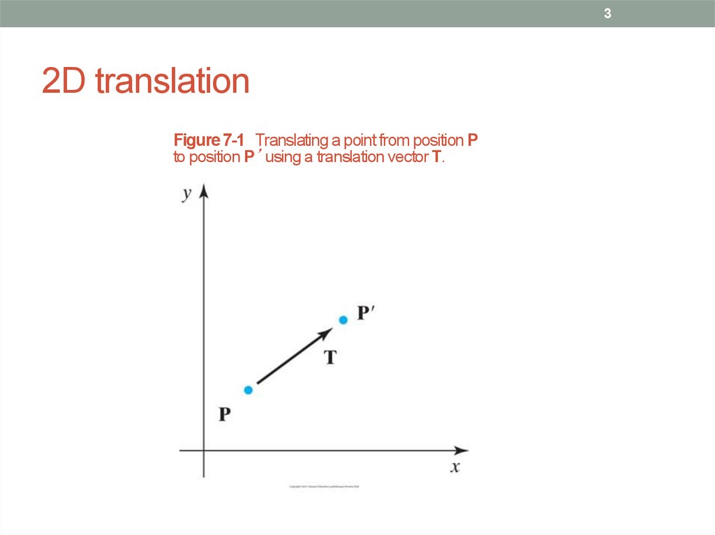
Figure 7-1 Translating a point from position P
to position P’ using a translation vector T.

4. 2D translation equations

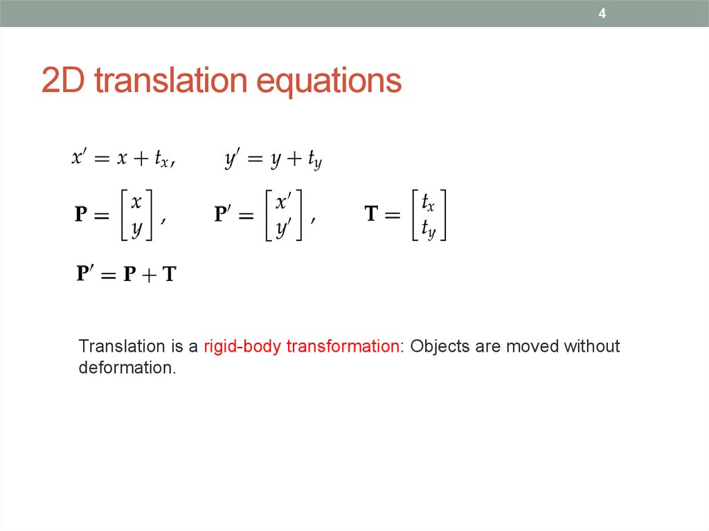
4
2D translation equations
Translation is a rigid-body transformation: Objects are moved without
deformation.

5. 2D translation example

5
2D translation example
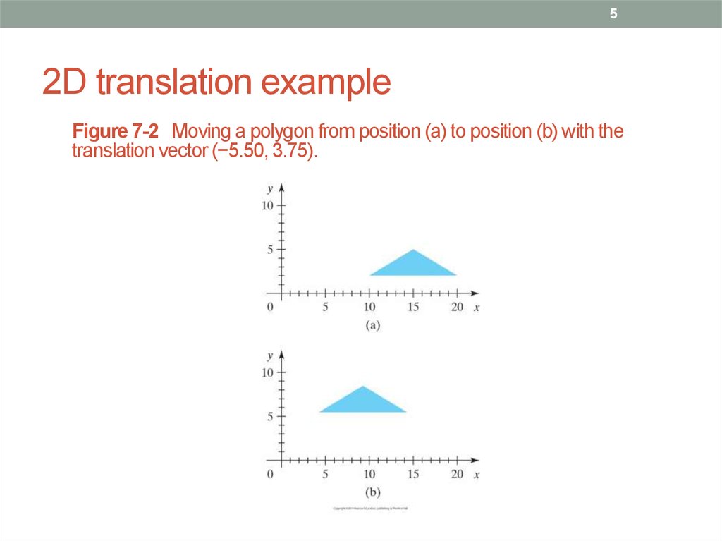
Figure 7-2 Moving a polygon from position (a) to position (b) with the
translation vector (−5.50, 3.75).

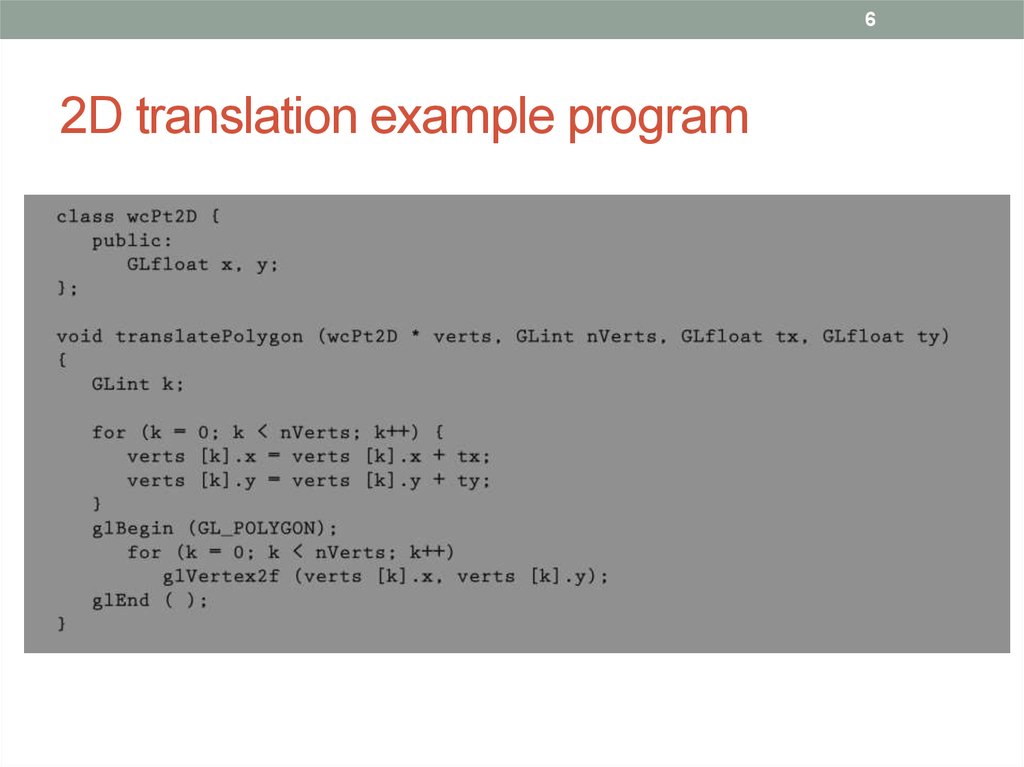
6. 2D translation example program

6
2D translation example program

7. 2D rotation

7
2D rotation
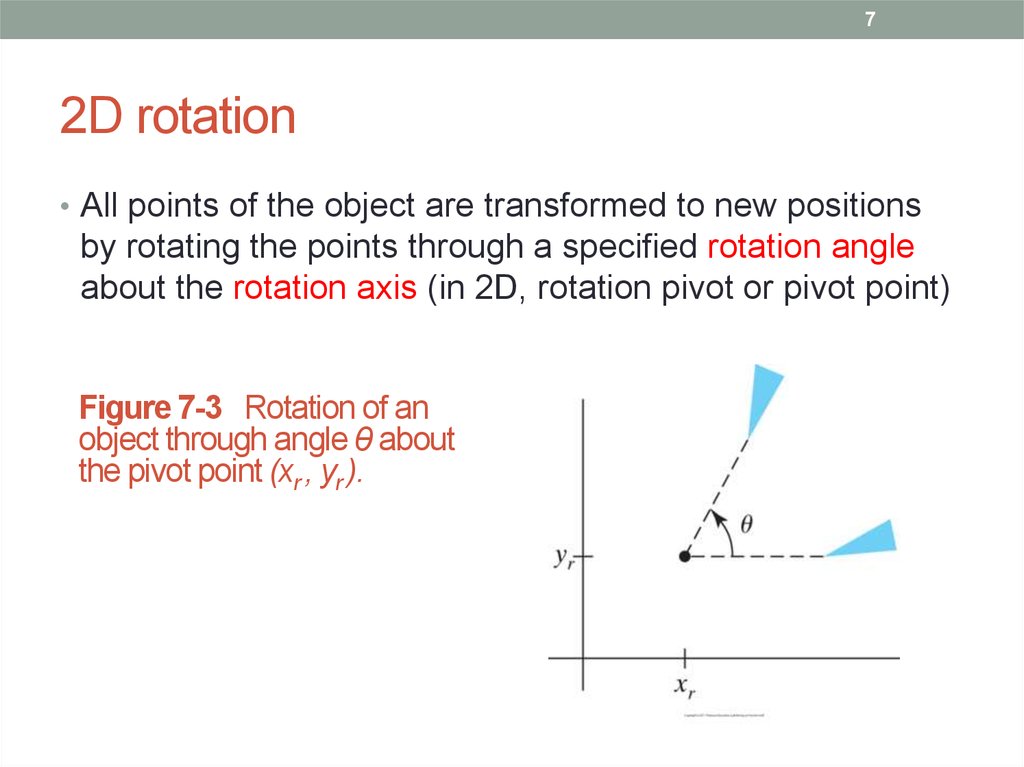
• All points of the object are transformed to new positions
by rotating the points through a specified rotation angle
about the rotation axis (in 2D, rotation pivot or pivot point)
Figure 7-3 Rotation of an
object through angle θ about
the pivot point (xr , yr ).

8. 2D rotation

8
2D rotation
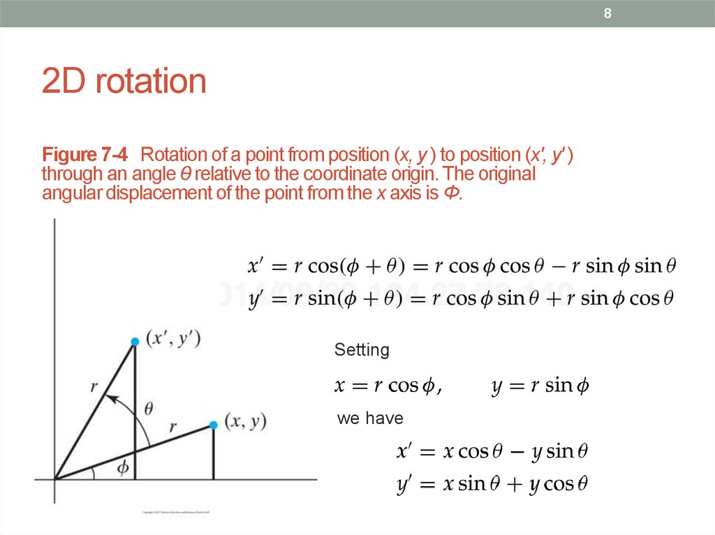
Figure 7-4 Rotation of a point from position (x, y ) to position (x', y' )
through an angle θ relative to the coordinate origin. The original
angular displacement of the point from the x axis is Φ.
Setting
we have

9. 2D rotation in matrix form

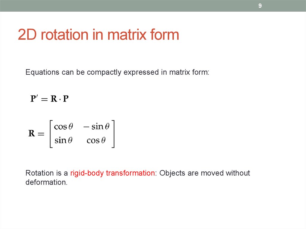
9
2D rotation in matrix form
Equations can be compactly expressed in matrix form:
Rotation is a rigid-body transformation: Objects are moved without
deformation.

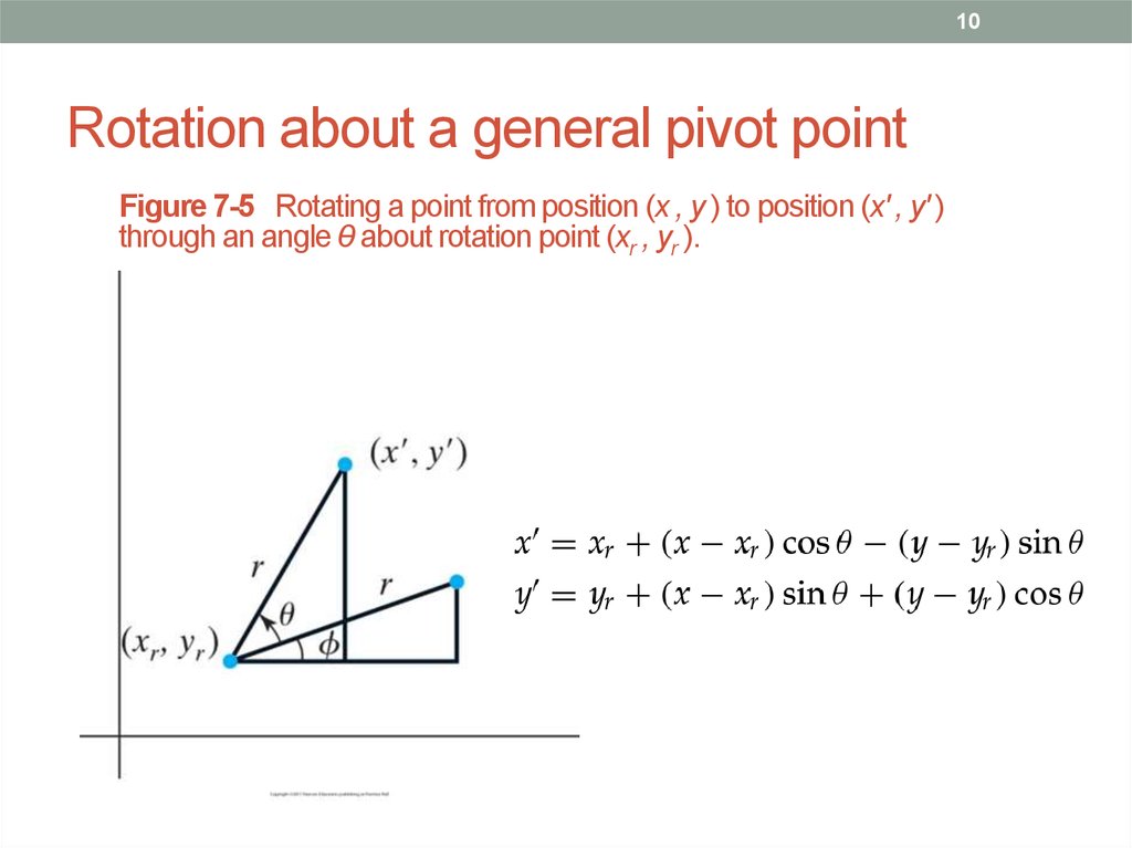
10. Rotation about a general pivot point

10
Rotation about a general pivot point
Figure 7-5 Rotating a point from position (x , y ) to position (x' , y' )
through an angle θ about rotation point (xr , yr ).

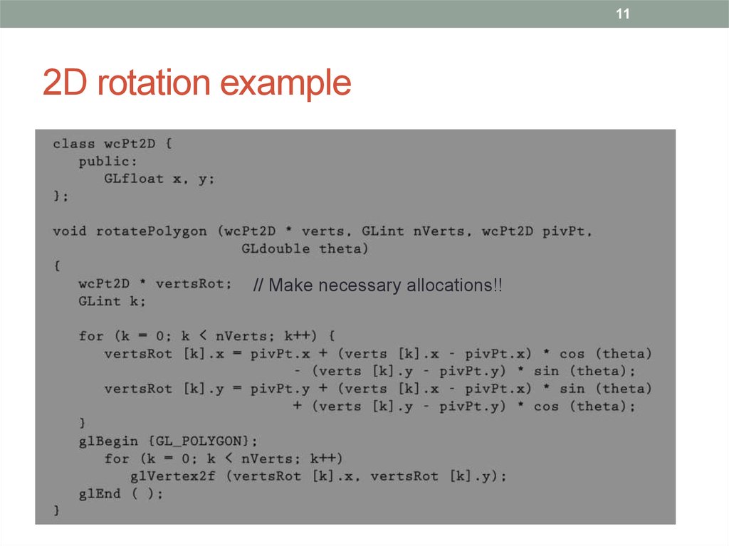
11. 2D rotation example

11
2D rotation example
// Make necessary allocations!!

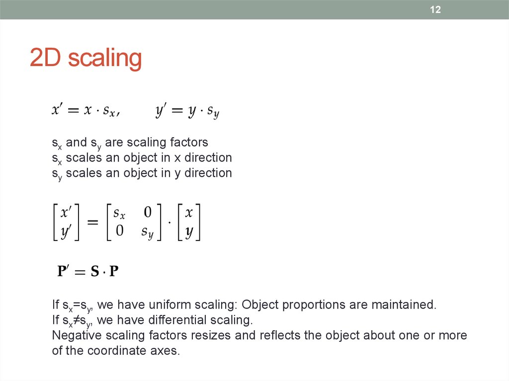
12. 2D scaling

12
2D scaling
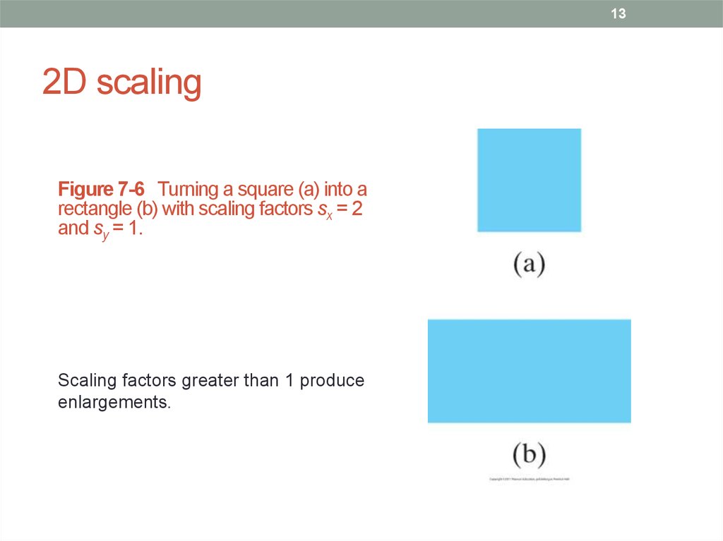
sx and sy are scaling factors
sx scales an object in x direction
sy scales an object in y direction
If sx=sy, we have uniform scaling: Object proportions are maintained.
If sx≠sy, we have differential scaling.
Negative scaling factors resizes and reflects the object about one or more
of the coordinate axes.

13. 2D scaling

13
2D scaling
Figure 7-6 Turning a square (a) into a
rectangle (b) with scaling factors sx = 2
and sy = 1.
Scaling factors greater than 1 produce
enlargements.

14. 2D scaling

14
2D scaling
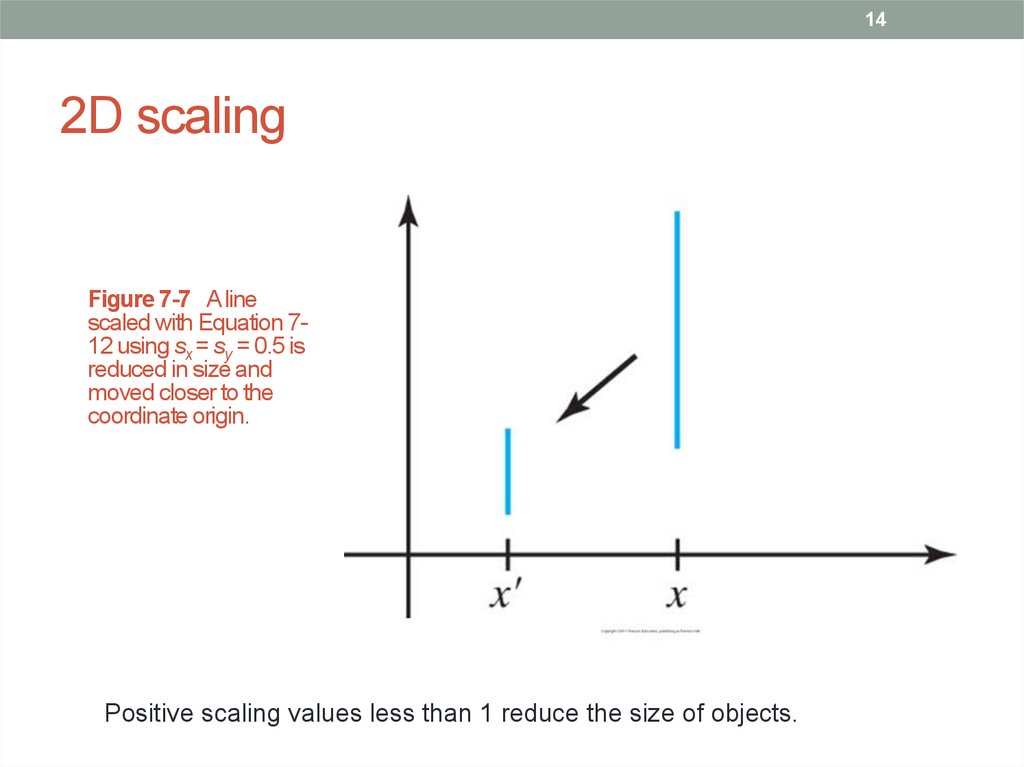
Figure 7-7 A line
scaled with Equation 712 using sx = sy = 0.5 is
reduced in size and
moved closer to the
coordinate origin.
Positive scaling values less than 1 reduce the size of objects.

15. Scaling relative to a fixed point

15
Scaling relative to a fixed point
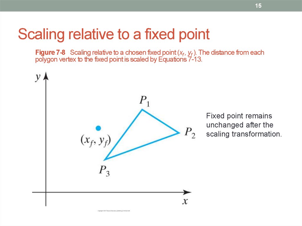
Figure 7-8 Scaling relative to a chosen fixed point (xf , yf ). The distance from each
polygon vertex to the fixed point is scaled by Equations 7-13.
Fixed point remains
unchanged after the
scaling transformation.

16. 2D scaling relative to a fixed point

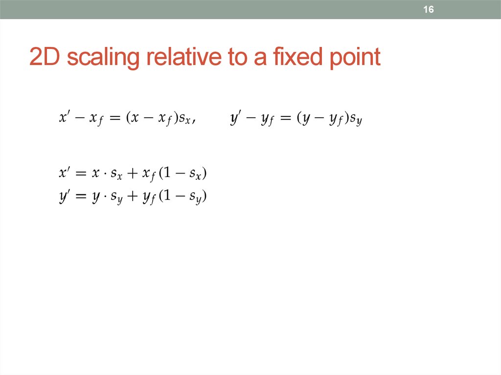
16
2D scaling relative to a fixed point

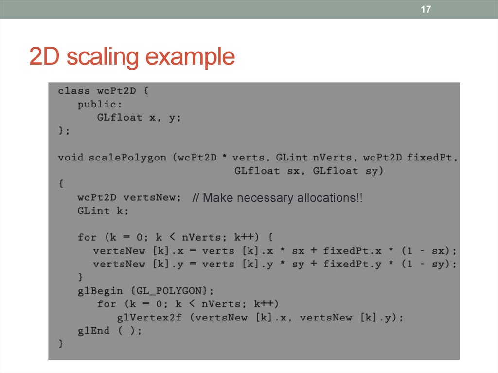
17. 2D scaling example

17
2D scaling example
// Make necessary allocations!!

18.

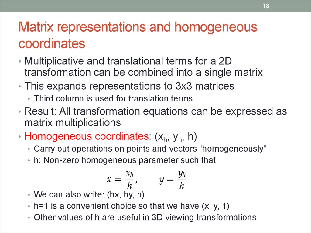
18
Matrix representations and homogeneous
coordinates
• Multiplicative and translational terms for a 2D
transformation can be combined into a single matrix
• This expands representations to 3x3 matrices
• Third column is used for translation terms
• Result: All transformation equations can be expressed as
matrix multiplications
• Homogeneous coordinates: (xh, yh, h)
• Carry out operations on points and vectors “homogeneously”
• h: Non-zero homogeneous parameter such that
• We can also write: (hx, hy, h)
• h=1 is a convenient choice so that we have (x, y, 1)
• Other values of h are useful in 3D viewing transformations

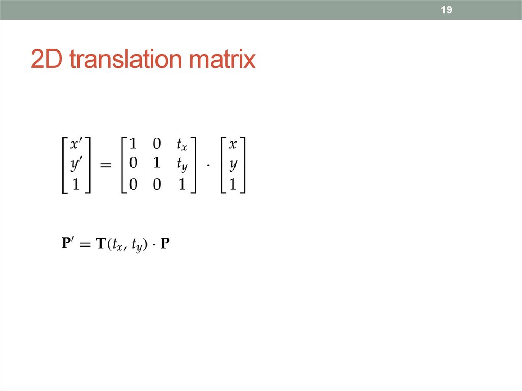
19. 2D translation matrix

19
2D translation matrix

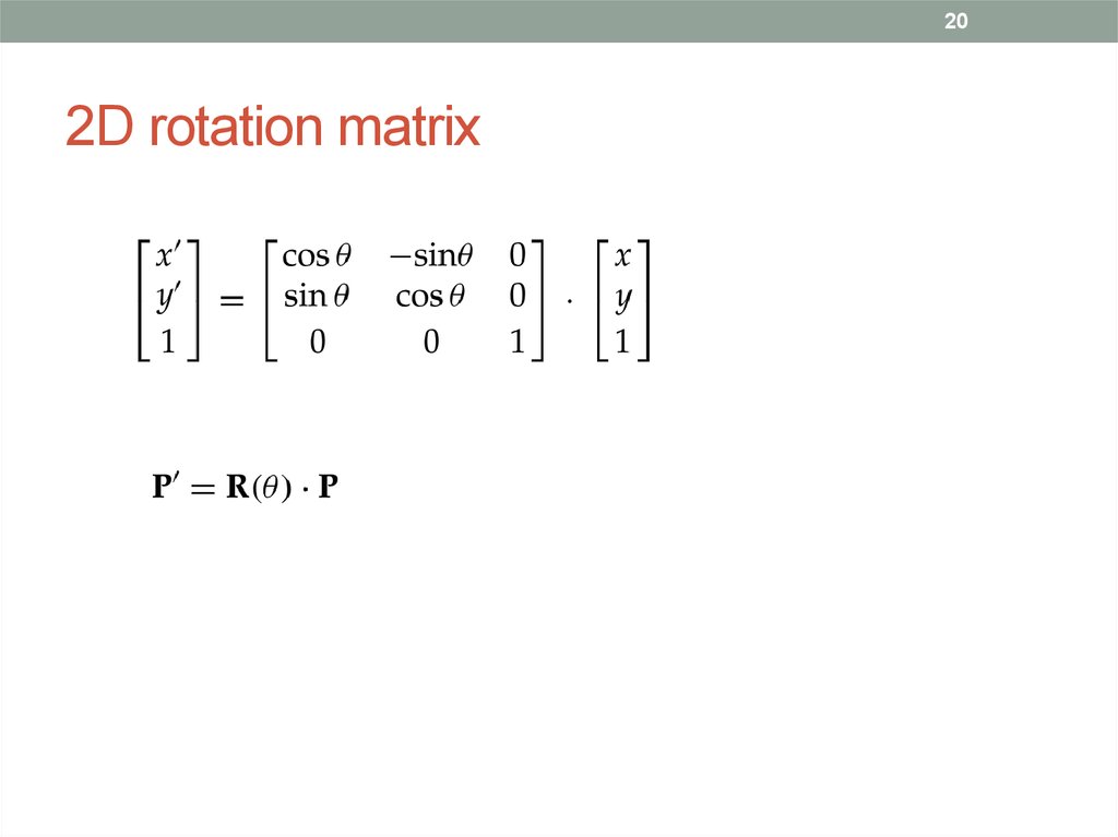
20. 2D rotation matrix

20
2D rotation matrix

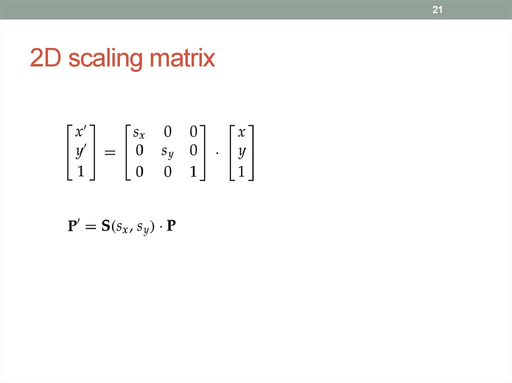
21. 2D scaling matrix

21
2D scaling matrix

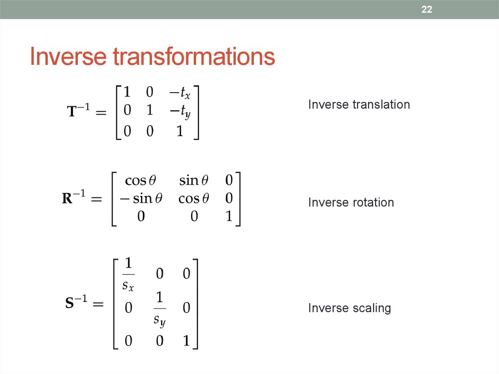
22. Inverse transformations

22
Inverse transformations
Inverse translation
Inverse rotation
Inverse scaling

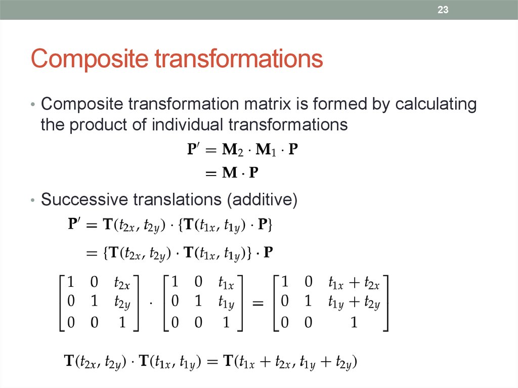
23. Composite transformations

23
Composite transformations
• Composite transformation matrix is formed by calculating
the product of individual transformations
• Successive translations (additive)

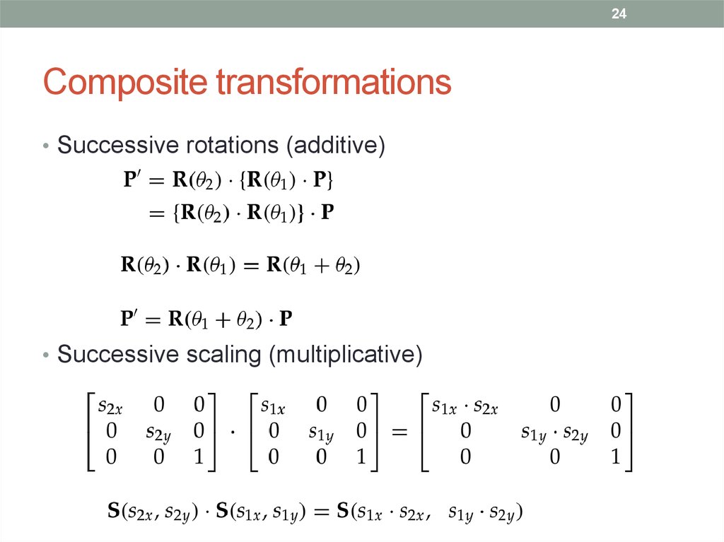
24. Composite transformations

24
Composite transformations
• Successive rotations (additive)
• Successive scaling (multiplicative)

25. 2D pivot-point rotation

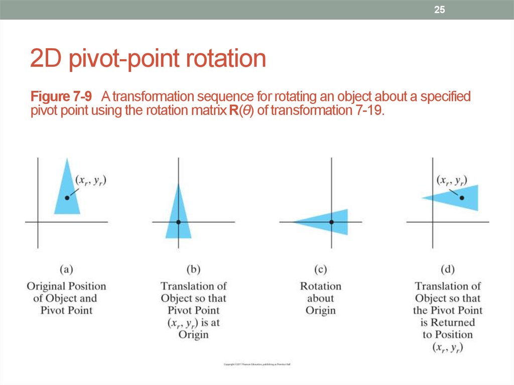
25
2D pivot-point rotation
Figure 7-9 A transformation sequence for rotating an object about a specified
pivot point using the rotation matrix R(θ) of transformation 7-19.

26. 2D pivot-point rotation

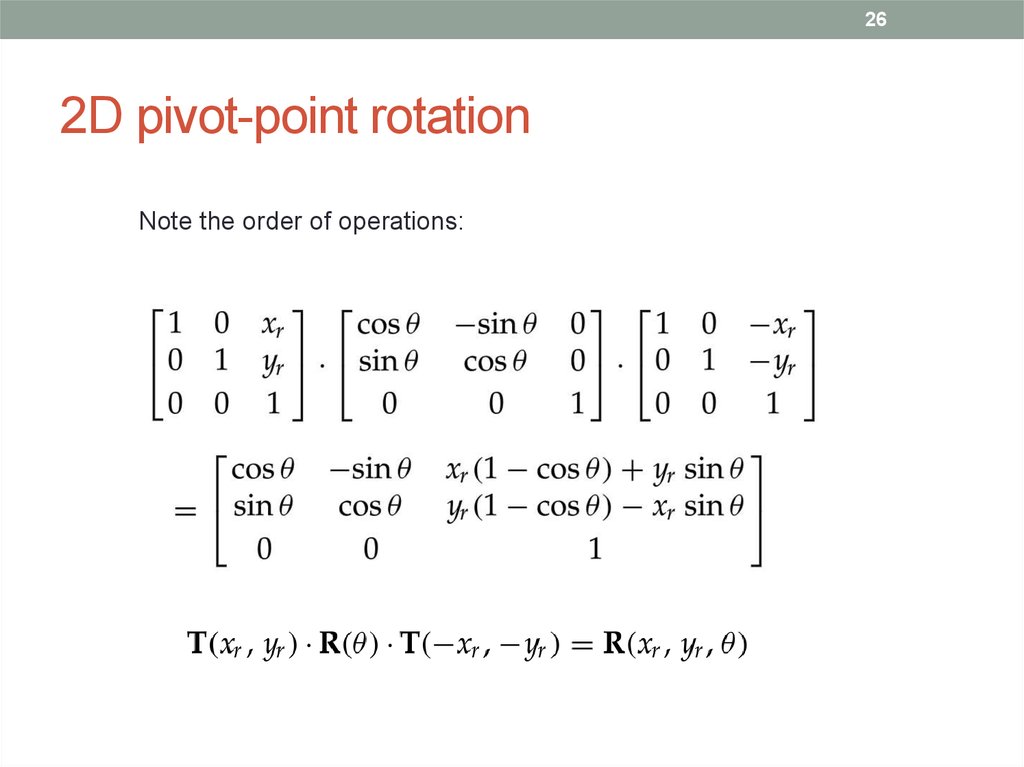
26
2D pivot-point rotation
Note the order of operations:

27. 2D fixed-point scaling

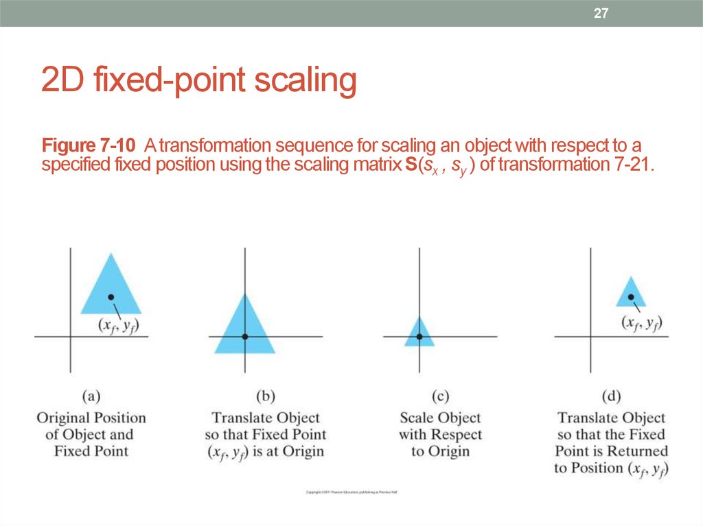
27
2D fixed-point scaling
Figure 7-10 A transformation sequence for scaling an object with respect to a
specified fixed position using the scaling matrix S(sx , sy ) of transformation 7-21.

28. 2D fixed-point scaling

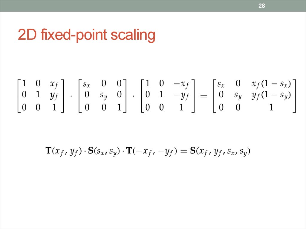
28
2D fixed-point scaling

29. Matrix concatenation properties

29
Matrix concatenation properties
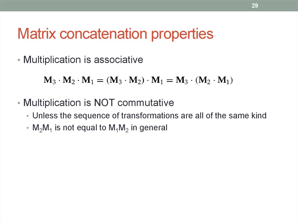
• Multiplication is associative
• Multiplication is NOT commutative
• Unless the sequence of transformations are all of the same kind
• M2M1 is not equal to M1M2 in general

30. Computational efficiency

30
Computational efficiency
• Formulation of a concatenated matrix may be more
efficient
• Requires fewer multiply/add operations
• Rotation calculations require trigonometric evaluations
• In animations with small-angle rotations, approximations (e.g.
power series) and iterative calculations can reduce complexity

31. Other transformations: reflection

31
Other transformations: reflection
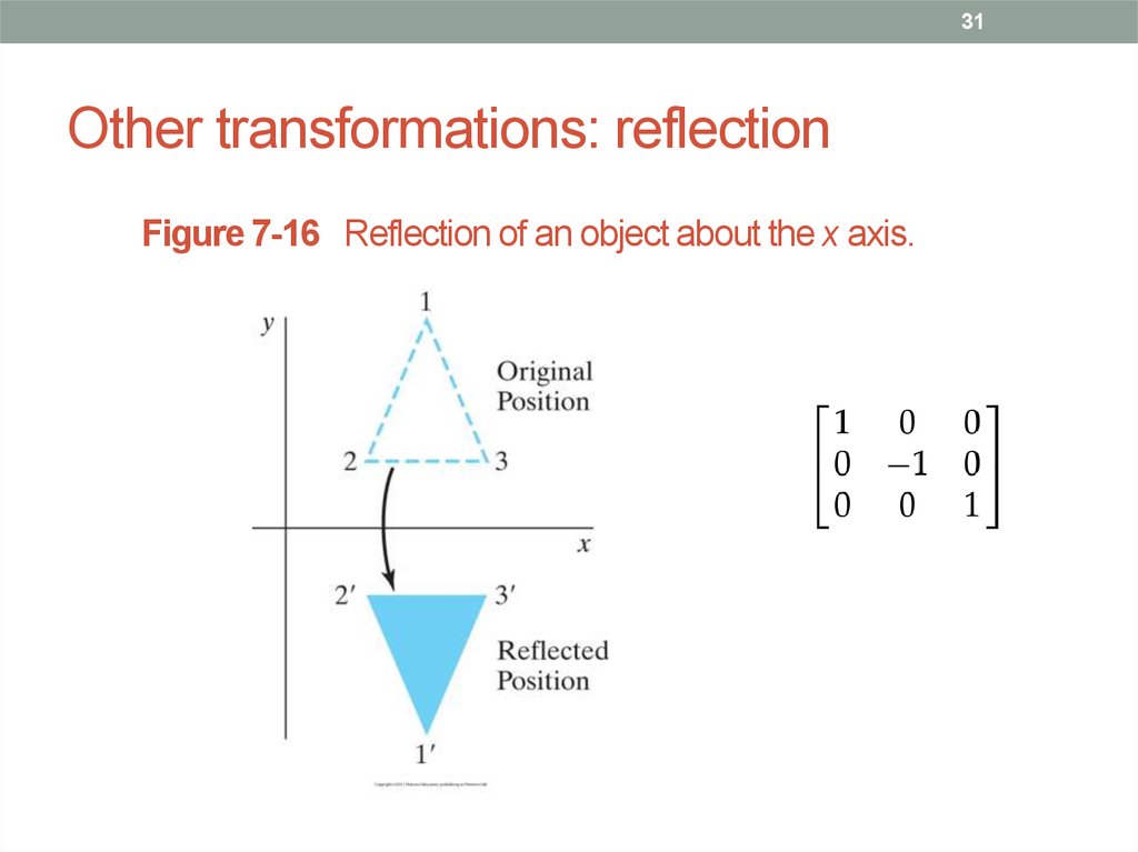
Figure 7-16 Reflection of an object about the x axis.

32. Reflection

32
Reflection
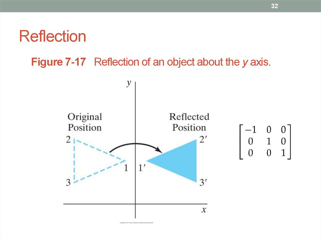
Figure 7-17 Reflection of an object about the y axis.

33. Reflection

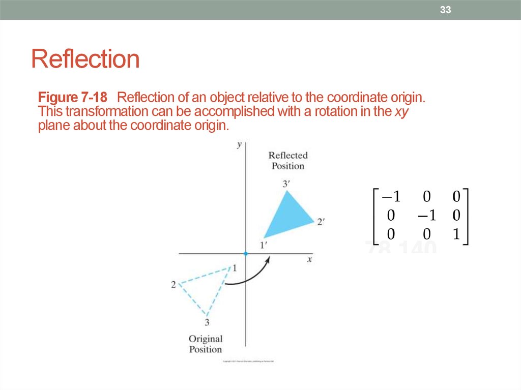
33
Reflection
Figure 7-18 Reflection of an object relative to the coordinate origin.
This transformation can be accomplished with a rotation in the xy
plane about the coordinate origin.

34. Reflection

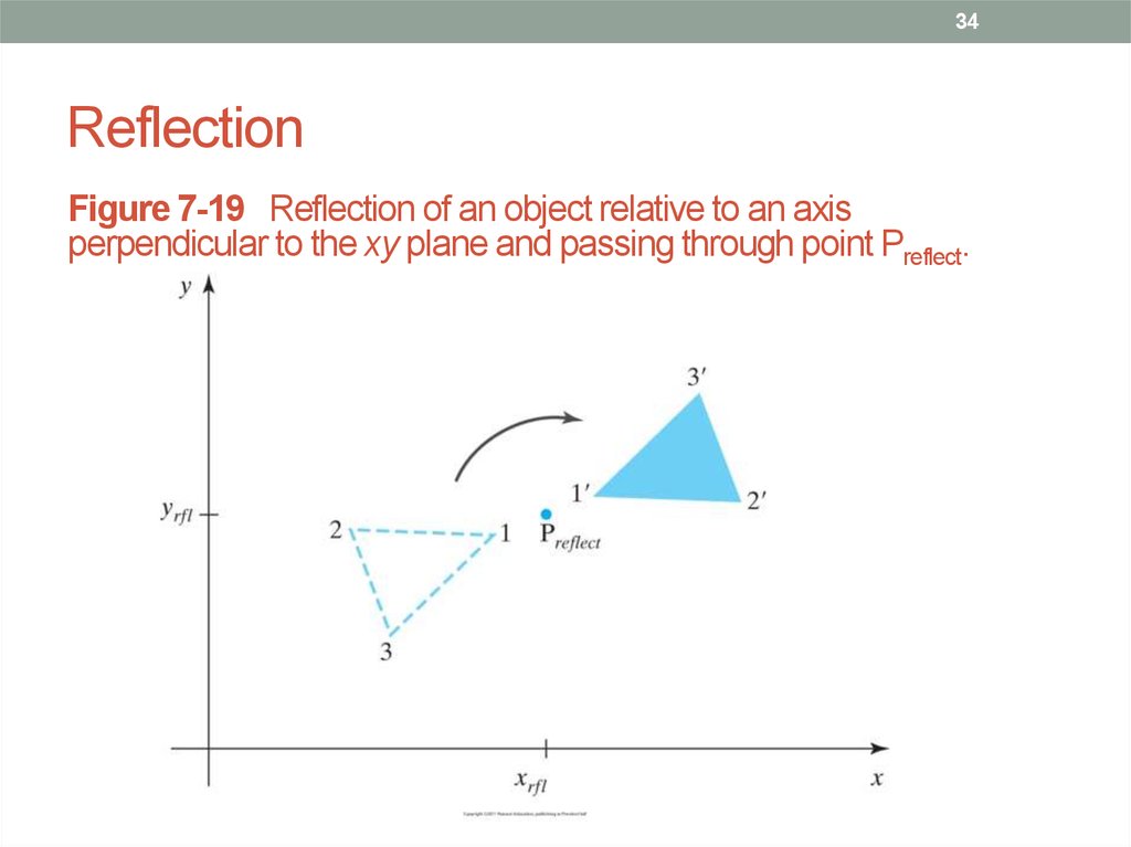
34
Reflection
Figure 7-19 Reflection of an object relative to an axis
perpendicular to the xy plane and passing through point Preflect.

35. Reflection

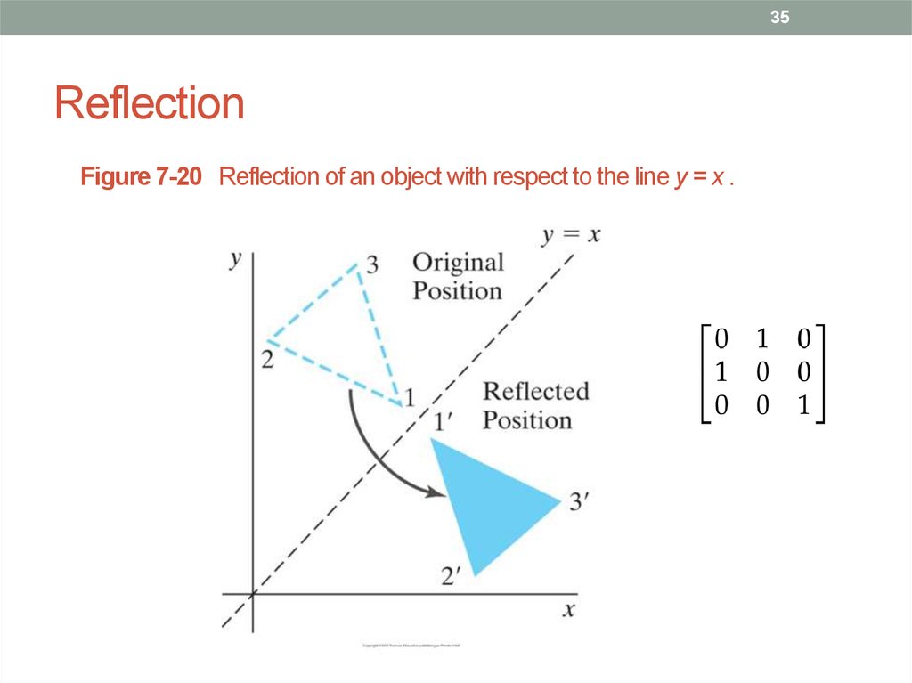
35
Reflection
Figure 7-20 Reflection of an object with respect to the line y = x .

36. Other transformations: shear

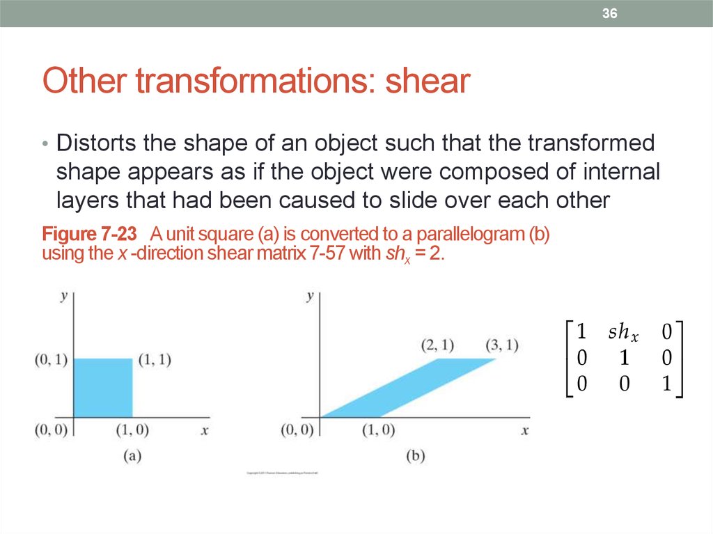
36
Other transformations: shear
• Distorts the shape of an object such that the transformed
shape appears as if the object were composed of internal
layers that had been caused to slide over each other
Figure 7-23 A unit square (a) is converted to a parallelogram (b)
using the x -direction shear matrix 7-57 with shx = 2.

37. Shear

37
Shear
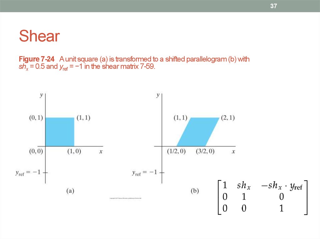
Figure 7-24 A unit square (a) is transformed to a shifted parallelogram (b) with
shx = 0.5 and yref = −1 in the shear matrix 7-59.

38. Shear

38
Shear
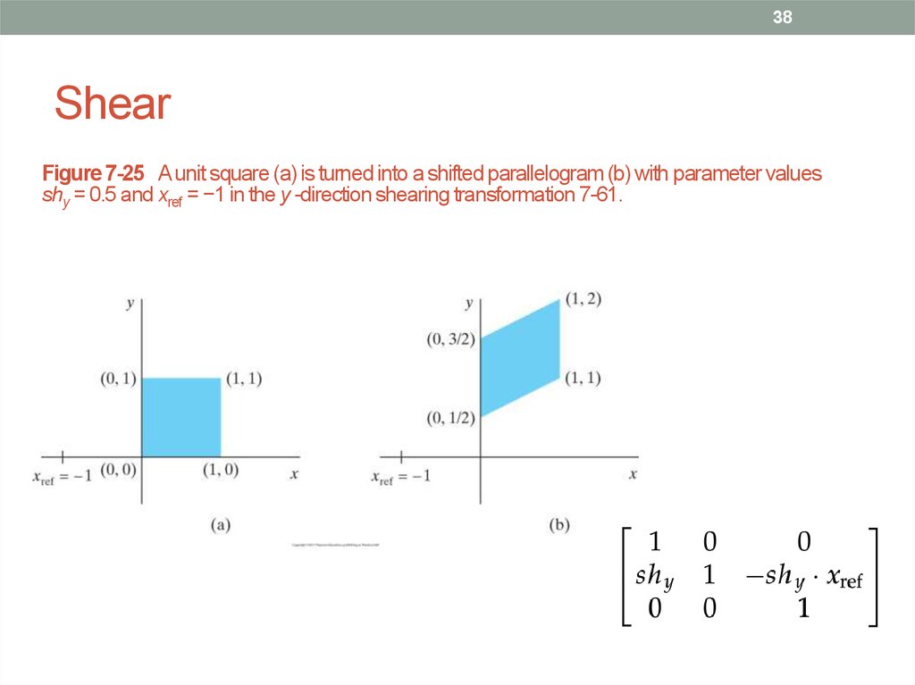
Figure 7-25 A unit square (a) is turned into a shifted parallelogram (b) with parameter values
shy = 0.5 and xref = −1 in the y -direction shearing transformation 7-61.

39. Transformations between 2D coordinate systems

39
Transformations between 2D coordinate
systems
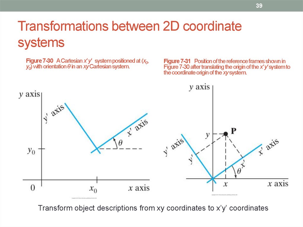
Figure 7-30 A Cartesian x' y' system positioned at (x0,
y0) with orientation θ in an xy Cartesian system.
Figure 7-31 Position of the reference frames shown in
Figure 7-30 after translating the origin of the x' y' system to
the coordinate origin of the xy system.
Transform object descriptions from xy coordinates to x’y’ coordinates

40. Transformations

40
Transformations
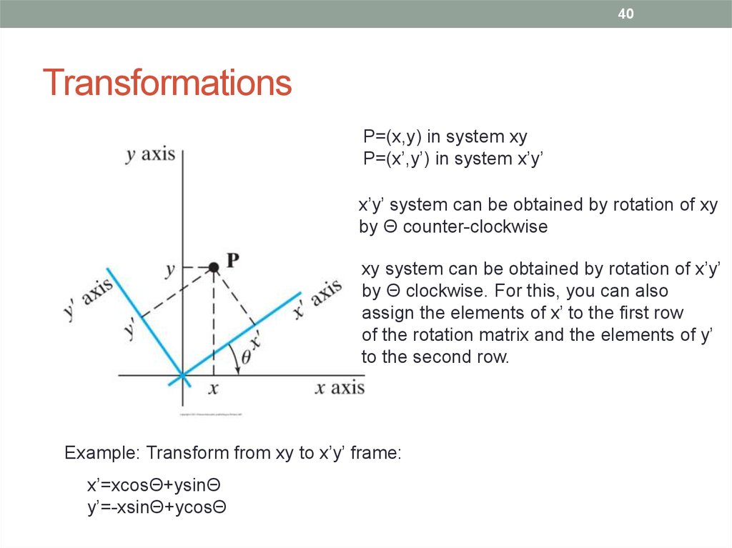
P=(x,y) in system xy
P=(x’,y’) in system x’y’
x’y’ system can be obtained by rotation of xy
by Θ counter-clockwise
xy system can be obtained by rotation of x’y’
by Θ clockwise. For this, you can also
assign the elements of x’ to the first row
of the rotation matrix and the elements of y’
to the second row.
Example: Transform from xy to x’y’ frame:
x’=xcosΘ+ysinΘ
y’=-xsinΘ+ycosΘ

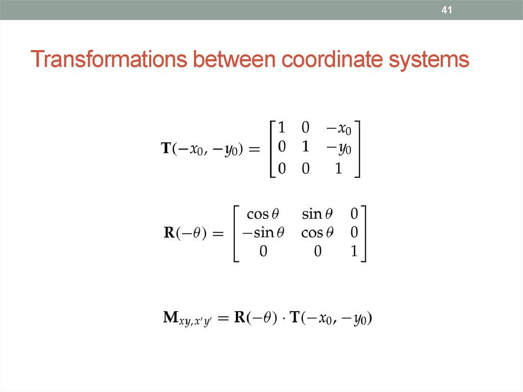
41. Transformations between coordinate systems

41
Transformations between coordinate systems

42. Alternative method

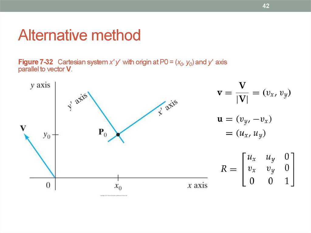
42
Alternative method
Figure 7-32 Cartesian system x' y' with origin at P0 = (x0, y0) and y' axis
parallel to vector V.

43. Transformations

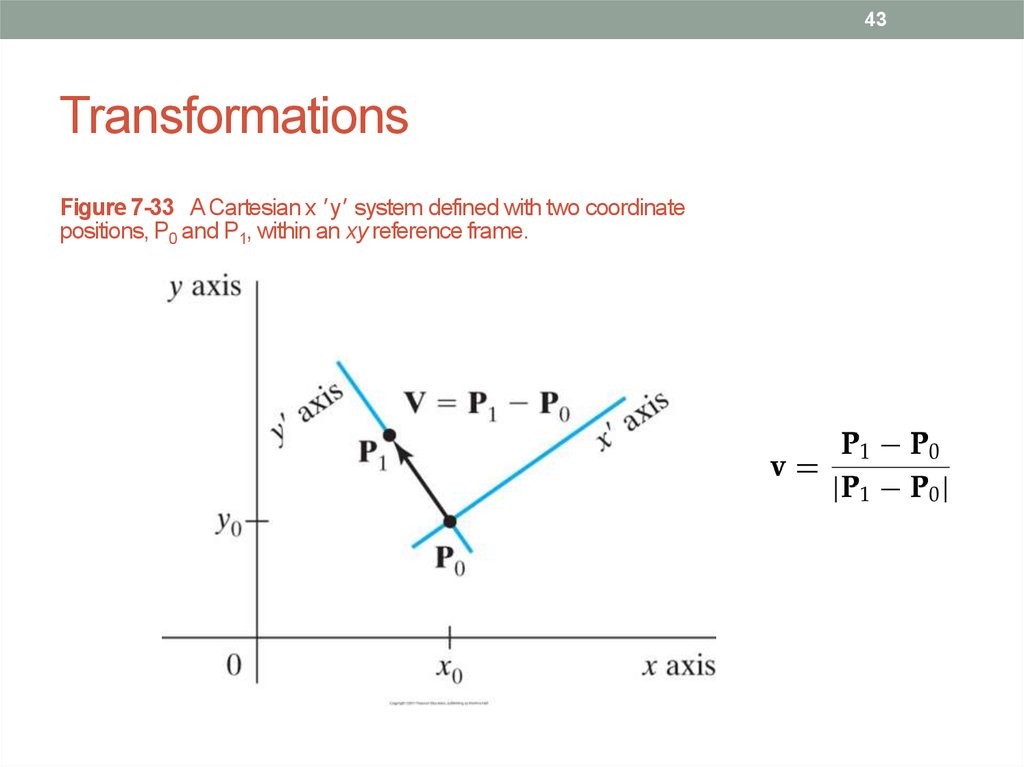
43
Transformations
Figure 7-33 A Cartesian x ' y' system defined with two coordinate
positions, P0 and P1, within an xy reference frame.

44. Example: Rotating points vs. rotating coordinate systems

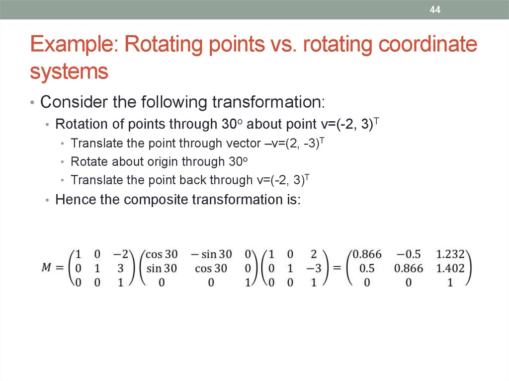
44
Example: Rotating points vs. rotating coordinate
systems
• Consider the following transformation:
• Rotation of points through 30o about point v=(-2, 3)T
• Translate the point through vector –v=(2, -3)T
• Rotate about origin through 30o
• Translate the point back through v=(-2, 3)T
• Hence the composite transformation is:

45. Example continued

45
Example continued
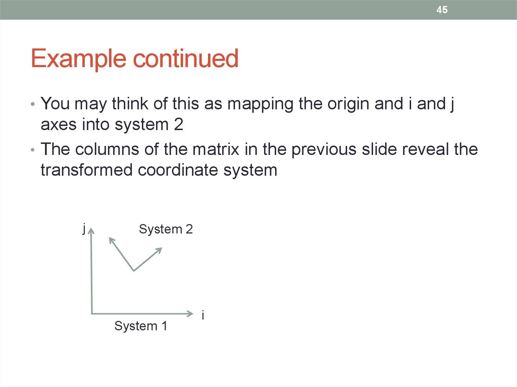
• You may think of this as mapping the origin and i and j
axes into system 2
• The columns of the matrix in the previous slide reveal the
transformed coordinate system
j
System 2
System 1
i

46. Example continued

46
Example continued
• Now consider the point P=(x(2),y(2),1)T in System 2
• What are the coordinates of this point expressed in terms
of the original System 1?
The answer is MP
For example, (1, 2, 1)T in System 2 lies at (1.098, 3.634,1)T
in System 1
Now, consider the point P=(x(1),y(1),1)T in System 1
What are the coordinates of this point expressed in terms
of System 2?
The answer is M-1P

47. OpenGL matrix operations

47
OpenGL matrix operations
• glMatrixMode ( GL_MODELVIEW )
• Designates the matrix that is to be used for projection
transformation (current matrix)
• glLoadIdentity ( )
• Assigns the identity matrix to the current matrix
• Note: OpenGL stores matrices in column-major order
• Reference to a matrix element mjk in OpenGL is a reference to the
element in column j and row k
• glMultMatrix* ( ) post-multiplies the current matrix
• In OpenGL, the transformation specified last is the one
applied first

48. OpenGL transformation example

48
OpenGL transformation example

49. OpenGL transformation example

49
OpenGL transformation example
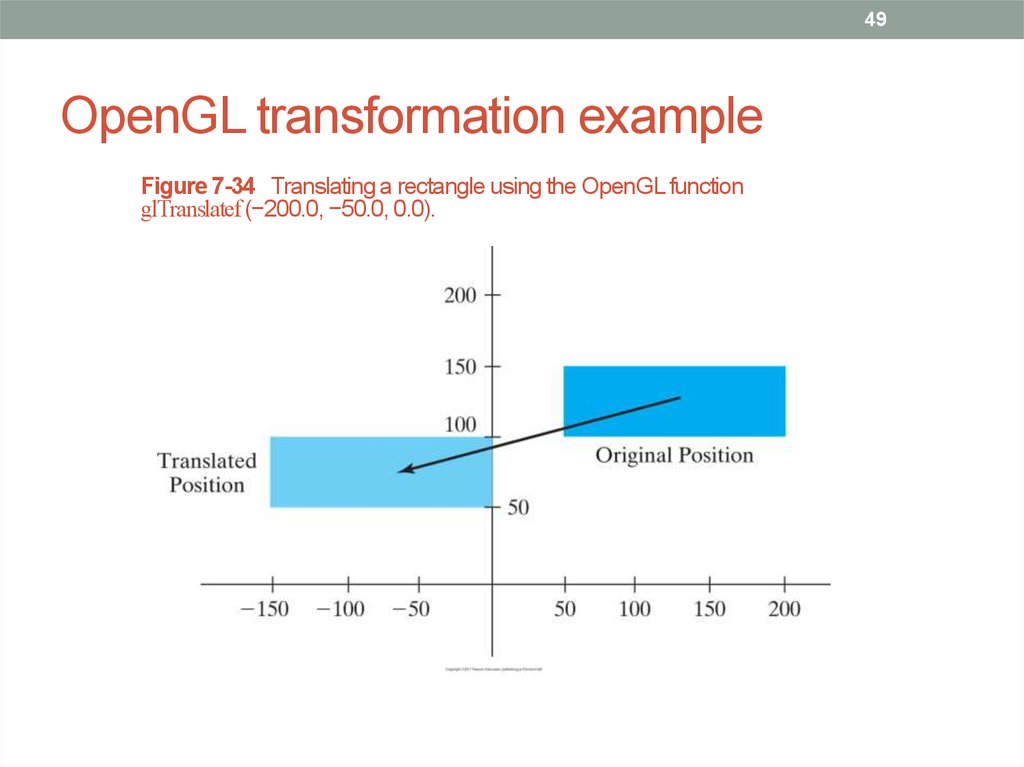
Figure 7-34 Translating a rectangle using the OpenGL function
glTranslatef (−200.0, −50.0, 0.0).

50. OpenGL transformation example

50
OpenGL transformation example
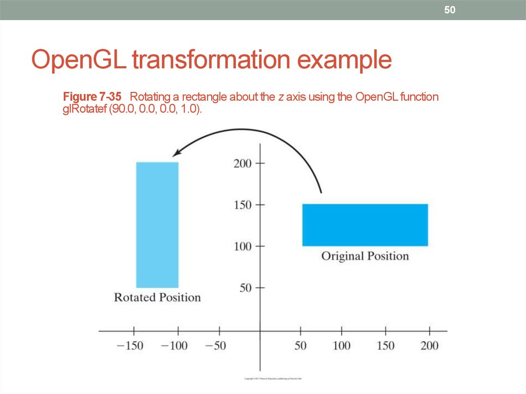
Figure 7-35 Rotating a rectangle about the z axis using the OpenGL function
glRotatef (90.0, 0.0, 0.0, 1.0).

51. OpenGL transformation example

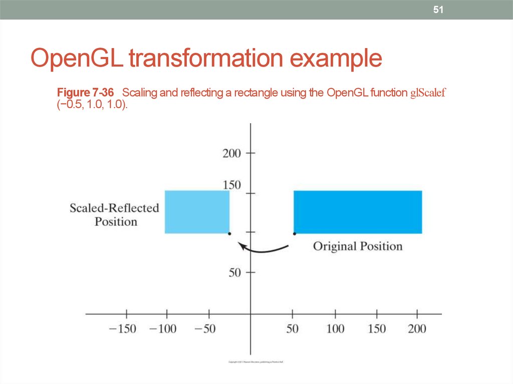
51
OpenGL transformation example
Figure 7-36 Scaling and reflecting a rectangle using the OpenGL function glScalef
(−0.5, 1.0, 1.0).